5 beautiful fractals animated in HTML5

Uses HTML5s canvas to create a framework that can be used to animate most fractals, particularly ones with L systems.

last modified 3 years, 8 months ago Maths HTML5

Fractals are the easiest place to go to for fun, simple and elegant programming projects, and so today, I have animated 5 different fractals in a HTML5 canvas and created a framework in which I can easily create others.

What is a fractal?

Fractals don’t have a very clear, simple, definition (unless you get into the concept of fractal dimension). However, most fractals share a couple of common properties.

Self-similarity - the fractal itself appears at other points in the fractal.
Infinite detail - this is almost a consequence of self-similarity.
Recursively defined - many (yet definitely not all) fractals can be defined in a recursive manner, building a shape up from smaller units. This is, once again, due to self similarity.

This makes them a perfect target for computer programs, as software can easily simulate these recursive definitions, and while infinite detail can’t be simulated in the real world, we can get very high levels of precise detail with computers.

An example of a fractal

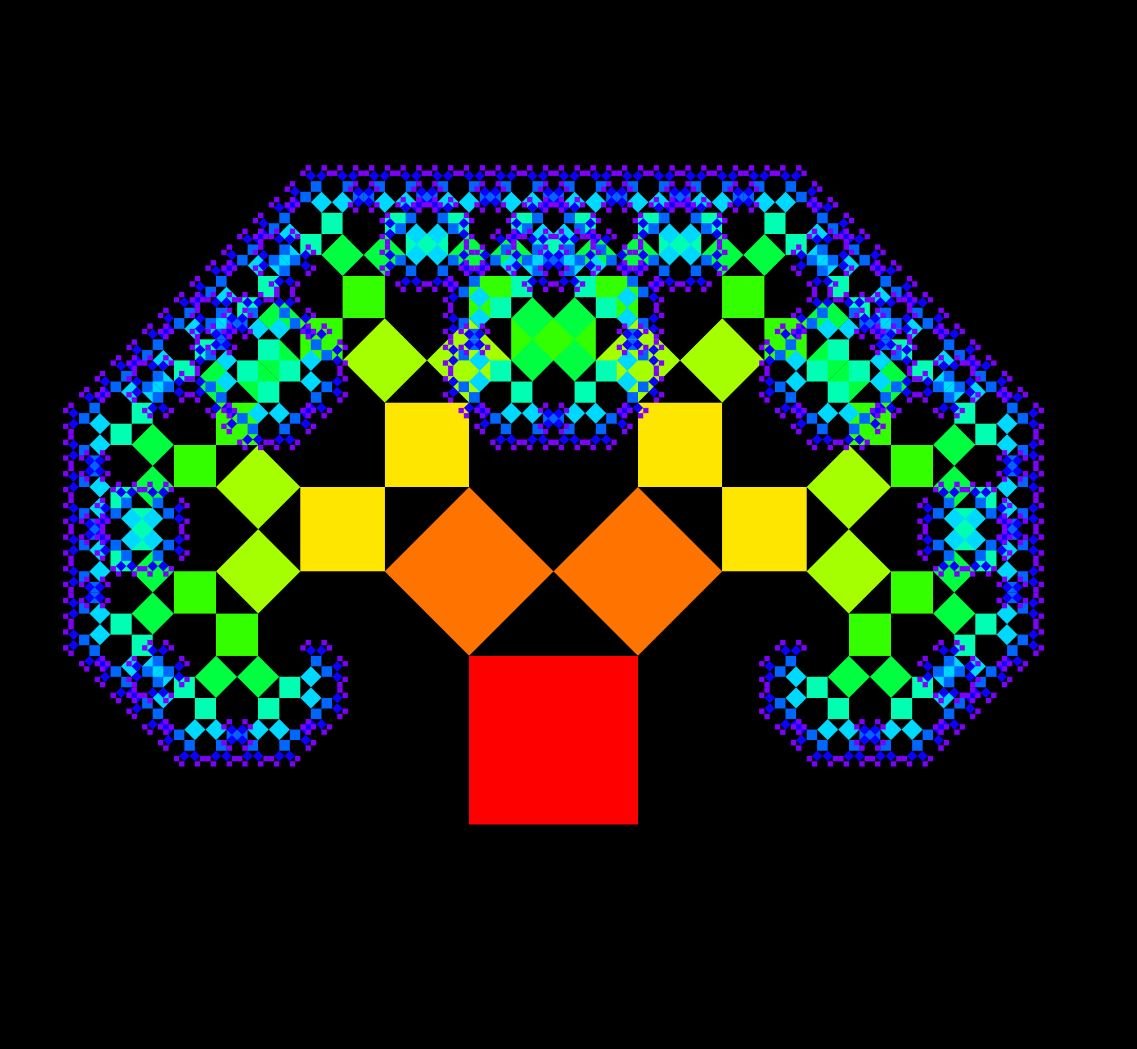
To explain the strategy I’m going to use to animate these, I’m going to be using the Pythagoras Tree as an example.

The Pythagoras tree is constructed of squares. It starts out at one square (the red one), and then a right angled triangle (in black here) is constructed on top of one of the squares. Then, two more squares are drawn on the two other sides of the right angled triangle. Then, the process repeats with these two squares.

This is once again the part where the article splits into two.
The next section is going to deal with technical details of implementation, while the section after is going to look at the more abstract concept of string rewriting and L systems.

A clean strategy for animating these fractals

In animating these fractals, the first thing that jumps out is the clear recursive nature of this problem.
We start with one square, and in the next step we end up with 2. This shows that we need some way to get one square to “spawn” two more in the next step.
In addition, we need to think about how we’re going to expand out the squares. We don’t want our squares to just pop into existence. We want some way to animate a square, and the most logical way to do this is to gradually increase its height.

Making our units

To make this more generalizable past the Pythagoras Tree, I’m going to call the squares units.
Each unit needs to be able to:

Draw itself at any point in its animation
Spawn its children

Therefore, each unit needs to implement both of these functions.

The units therefore need to carry some sort of metadata, namely coordinates so that they can be correctly positioned and drawn, and maybe some extra data: in the case of the Pythagoras Tree, the depth so that they can be drawn in different colours.

To deal with drawing at any point in the animation, each unit is going to have a function draw that draws the unit on the canvas. The draw function is going to take a parameter step that ranges from 0 to 1 showing the progress in the animation. The value of step can also be -1 indicating that this unit is not being animated, but this will become more clear later.

The whole unit for the Pythagoras Tree is shown below.
Note that the following code uses Three.js’s Vector2 library.

function pythagtree(coords, depth) {
    let sidevec = new Vector2().subVectors(coords[1], coords[0])
    let perpvec = sidevec.clone().rotateAround(new Vector2(0, 0), Math.PI / 2);
    let side = sidevec.length();
    let draw = (step) => {
        if (step == -1) step = 1;
        // calculate corner vectors
        let sidevector = perpvec.clone().multiplyScalar(step);
        let point1 = coords[0].clone().add(sidevector);
        let point2 = point1.clone().add(sidevec);
        ctx.fillStyle = "hsl(" + (((270 / fullDepth) * depth) + 0) + ",100%,50%)";

        ctx.beginPath();
        ctx.moveTo(...coords[0].toArray());
        ctx.lineTo(...point1.toArray());
        ctx.lineTo(...point2.toArray());
        ctx.lineTo(...coords[1].toArray());
        ctx.lineTo(...coords[0].toArray());
        ctx.fill();
    }
    // once the drawer is complete, this will be called to make the children for next paints
    let makeChildren = () => {
        let rotpoint = sidevec.clone().rotateAround(new Vector2(0, 0), Math.PI / 4).multiplyScalar(1 / Math.sqrt(2)).add(perpvec).add(coords[0]);
        let children = [pythagtree([coords[0].clone().add(perpvec), rotpoint], depth + 1), pythagtree([rotpoint, coords[1].clone().add(perpvec)], depth + 1)]
        return children;
    }
    return { "draw": draw, "makeChildren": makeChildren };
}

The fractal runner

Now that we have a unit, we need something that will execute the whole cycle of drawing and spawning new units.

To render a frame, we need to:

Clear the previous frame
Draw the background (if any)
Draw any units we aren’t currently animating.
Check our progress in the step
- If the step is complete, we need to spawn children of each unit and call a callback
Draw any units we’re currently animating
- We may want to add a way to easily add an ease-in/ease-out, so I add a timing function parameter that will be explained later.
Set the frame to be redrawn in the next browser frame
End the animation if it is complete.

This is completely implemented in the Fractal class, shown below.

function animate_linear(x) { return x }
function animate_quadratic(x) { return 1 - Math.pow(1 - x, 2) }
 
class Fractal {
    constructor(options) {
        this.clear = options.clear;
        this.drawBackground = options.drawBackground;
        this.timingFunc = options.timingFunc;
        this.endInProgress = options.endInProgress === true;
        this.cback = options.callback == undefined ? () => { } : options.callback;
        this.finish = options.finishedCb == undefined ? () => { } : options.finishedCb;
        this.stagestep = options.stagestep == undefined ? () => { } : options.stagestep;
        this.animcontext = {
            "completeds": [],
            "inprogress": [],
            "progress": 0,
            "framecount": 45,
            "currDepth": 0,
            "maxDepth": 7,
            "animating": true
        }
    }
 
    animate() {
        if (this.animcontext.animating) {
            window.requestAnimationFrame(() => { this.animate() });
        }
        // clear it
        this.clear();
        this.drawBackground();
        // do housekeeping
        if (this.animcontext.progress == (this.animcontext.framecount)) {
            this.animcontext.progress = 0;
            this.animcontext.currDepth += 1;
            if (this.animcontext.currDepth <= this.animcontext.maxDepth) {
                this.stagestep();
            }
            // move our completeds out
            let newinprogress = [];
            this.animcontext.inprogress.forEach((x) => { newinprogress.push(...x.makeChildren()) })
            this.animcontext.completeds.push(...this.animcontext.inprogress);
            this.animcontext.inprogress = newinprogress;
        }
        // now make the background
        this.animcontext.completeds.forEach((x) => { x.draw(-1); })
        if (this.animcontext.currDepth > this.animcontext.maxDepth) {
            this.animcontext.animating = false;
            if (!this.endInProgress) {
                this.finish();
                return;
            }
        }
        // now draw the animations
        this.animcontext.inprogress.forEach((x) => { x.draw(this.timingFunc(this.animcontext.progress / this.animcontext.framecount)) })
        this.animcontext.progress += 1;
 
        this.cback();
 
        if (this.animcontext.currDepth > this.animcontext.maxDepth) {
            this.animcontext.animating = false;
            this.finish();
            return;
        }
    }
}

The class internally maintains two lists, one of all units that are currently being animated and one of all units that have their animations completed.

To run an animation, I simply create an instance of the Fractal class, adjust some parameters, and put an initial unit in the “currently being animated” list. Then, calling the animation function does the rest of the work for me.

Playing with the timing parameters

Remember the previously mentioned timing parameter?
These are the two functions called animate_linear and animate_quadratic.

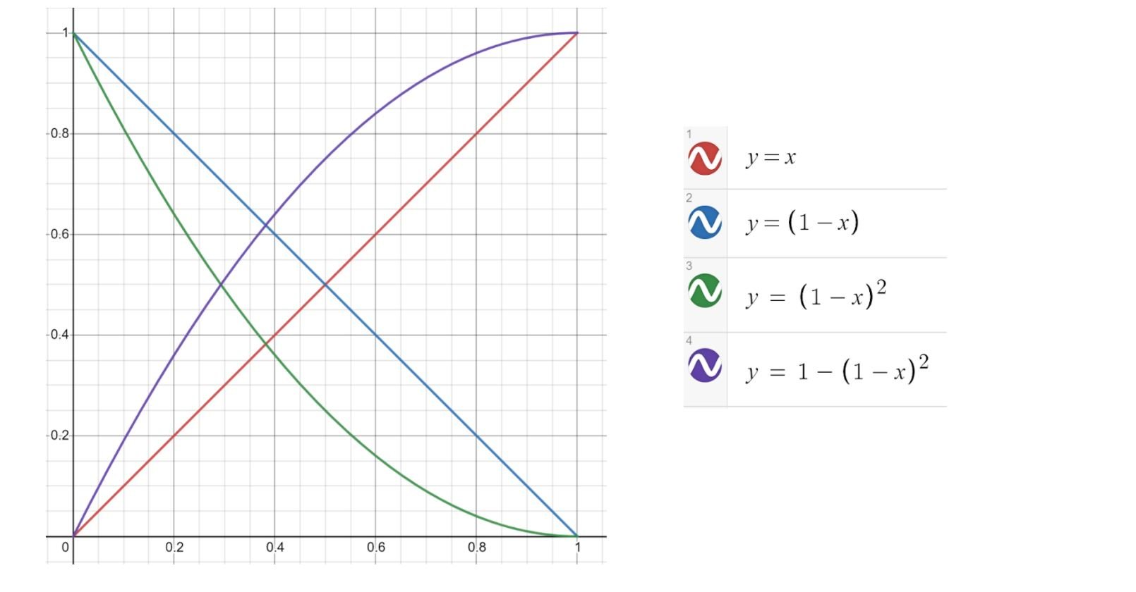
After I created the animations, I wanted the progress of the animation to start out fast and finish slowly. To do this, I tweak the input to the draw function of the units before passing it to the unit.

The input originally moves linearly between 0 and 1 - the purpose of the timing function is to introduce some non-linearity.

To do an ease out, I use the timing function \(1 - (1 - x)^2\).
This creates an ease out, as shown in the following Desmos plots.

L-systems and string replacement

This strategy for fractal generation typically works for anything that can be represented as an L-system.

L-systems are methods of generating infinite sequences or graphics with replacement rules on a few states. L-systems have a grammar of symbols, rules for replacing symbols with other symbols and a method to turn symbols into something visible.
For example, consider the Koch curve. This is the fractal shown below:

This can be represented as an L-system.
The grammar will be F, L, R.
The method gives F, L and R meanings. When processing a string, F will mean move forwards, L will mean turn left 60 degrees and R will mean turn right 120 degrees.
The replacement rules are:
L => L
R => R
F => FLFRFLF

To create the curve, we start with an axiom. The axiom in this case is F, drawing a single straight line.
In the first stage, we apply the replacement rules to the axiom string to get FLFRFLF, drawing the following:

In the next iteration, we apply the same replacement rules to the previous string FLFRFLF, giving us FLFRFLFLFLFRFLFRFLFRFLFLFLFRFLF as the next string. This draws the following:

Iterating this gives the Koch curve.

This idea of replacement works really well with the spawning recursion idea of the program.