Numerical evolution of dynamical systems, and Lagrangian mechanics

The motivation for this article once again comes from the MIT Motorsports team. I have always wanted to model the full transient performance of the car, and I have enjoyed investing time into designing and developing a variety of models for this task.$$

The previous article showed a method to analyse very generic dynamical systems by automatically identifying degrees of freedom, and then evaluating the dynamics in these degrees of freedom using an extension of D'Alemberts principle. However, I decided to move away from this method for the task of vehicle design for a few reasons:

1. The computation in the previous method is too expensive, and simulation can end up being prohibitively slow. The method also has some issues with numerical instability
2. It is very difficult to make design decisions from such a complex model. The previous method took all suspension geometry as an input, but I think I am still a ways away from being able to directly optimize the full car's suspension geometry.

To get around these issues, I decided to use a simpler model that models all complexities of suspension e.t.c. as simple springs. This (for now) does not account for progressive motion ratios and other higher level complexities, but still provides quite a comprehensive and easy to tweak model of the full car.

However, I want to emphasize that this article is not an article on vehicle design. This is an article on physics and numerical computation, so I will not go into deep details on how the car model itself works (maybe some other time!). This is an article on Lagrangian mechanics, a powerful tool to analytically evaluate dynamic systems, and how it can be applied in a computational context.

How Lagrangian mechanics works

Lagrangian mechanics is incredibly powerful in dynamics evaluation, described as "the sledgehammer of dynamics". However, a lot of the information on this topic is heavily fragmented and doesn't, in my opinion, give satisfying explanations on how the Euler-Lagrange equations work. In this first section, I will look at the Euler-Lagrange equations and how they can be derived from first principles.

Euler-Lagrange equations

One thing many mechanics students may not know is that the Euler-Lagrange equations are actually a result from variational calculus, and can be derived without a drop of physics. Consider some once-differentiable variable $q$ and some "time variable" $t$. $q$ can be (and usually is a vector) so we will denote it as $\overrightarrow{q}$.

The goal of the calculus of variations in this case in this case is to find some function $\overrightarrow{q}(t)$ that is a stationary point of the following integral:
$$S[q]={\int }_a^{b}L(t,\overrightarrow{q}(t),\dot{\overrightarrow{q}}(t))\text{d}t$$
subject to the condition that $\overrightarrow{q}(a)$ is some constant $\overrightarrow{A}$ and $\overrightarrow{q}(b)=\overrightarrow{B}$.
Here, $L$ is any twice differentiable function on $t$, $\overrightarrow{q}(t)$ and $\dot{\overrightarrow{q}}(t)$. $a,b$ are arbitrary constants.

This might seem a bit abstract, so to provide some intuition, you can think of $\overrightarrow{q}(t)$ as being the state of some system over time. The constraints $\overrightarrow{q}(a)=\overrightarrow{A}$ and $\overrightarrow{q}(b)=\overrightarrow{B}$ means that $\overrightarrow{q}$ starts and ends at some predefined states at times $a$ and $b$. You can think of $L(t,\overrightarrow{q}(t),\dot{\overrightarrow{q}}(t))$ being the "cost" of the current state and its rate of change at time $t$, and the goal of the whole problem is to find out the "route" of $\overrightarrow{q}(t)$ between times $a$ and $b$ in a way that minimizes the total cost given by $L$ over the route.

This paradigm of minimizing a cost over a route shows up sometimes in physics. One that many readers may be familiar with is Fermat's principle, which states that light takes the path which minimizes the time taken between two points. (This doesn't immediately work with this formulation, as the "time variable" becomes distance, but you get the general jist)The Euler-Lagrange equations don't allow you to find a global minimum (calculus in general can't do that very well) but they can give some information on a stationary point of $S$. A "stationary point" here means that if I have some path $\overrightarrow{q}(t)$ and I slightly perturb it while continuing to follow the constraints, $S$ will not change to the first order. This often means that the path found is the path that minimizes $S$.

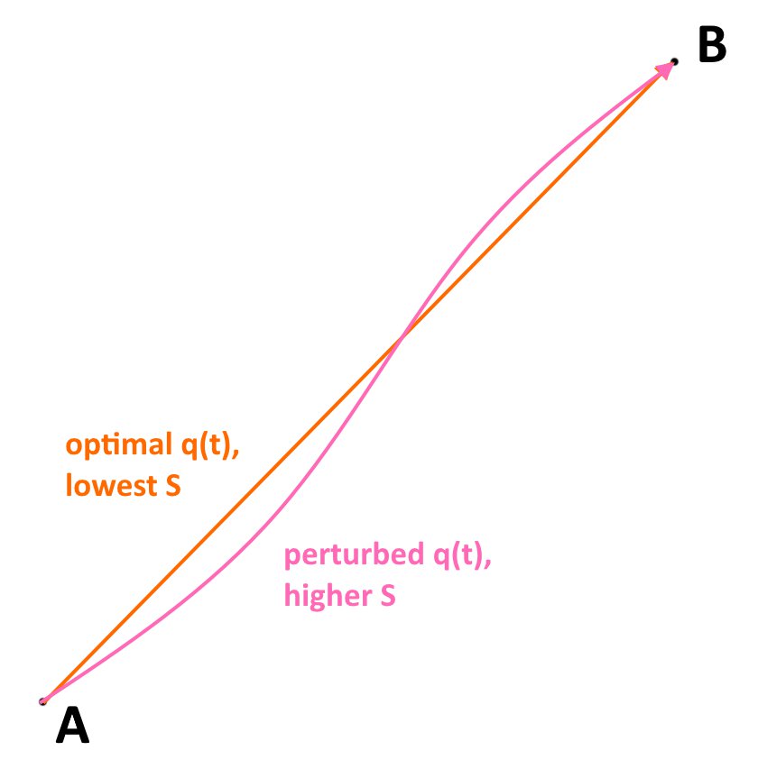
The Euler Lagrange equations are actually derived by following this exact idea numerically. Suppose that ${\overrightarrow{q}}^{\ast }(t)$ is my optimal path. Consider an alternative path given by ${\overrightarrow{q}}^{\ast }(t)+\epsilon \overrightarrow{\eta }(t)$, given the constraints that $\overrightarrow{\eta }(a)=\overrightarrow{\eta }(b)=\overrightarrow{0}$ to ensure that the new path continues to satisfy $\overrightarrow{q}(a)=\overrightarrow{A}$ and $\overrightarrow{q}(b)=\overrightarrow{B}$. At a stationary point, no matter what $\overrightarrow{\eta }(t)$ is, we expect
$$\frac{\text{d}}{\text{d}\epsilon }S[q^{\ast }+\epsilon \eta ]=\frac{\text{d}}{\text{d}\epsilon }{\int }_a^{b}L(t,{\overrightarrow{q}}^{\ast }(t)+\epsilon \overrightarrow{\eta }(t),\dot{{\overrightarrow{q}}^{\ast }}(t))+\epsilon \dot{{\overrightarrow{\eta }}^{\ast }}(t))\text{d}t=0$$
This means that for small $\epsilon$, slightly changing the path by $\eta$ will, to first order, not change $S$ i.e. we have found a stationary point of $S$.
Bring the derivative inside the integral (as the integral is in a different variable) and then differentiate $L$:
$$\begin{array}{rl}\frac{\text{d}}{\text{d}\epsilon }S[q^{\ast }+\epsilon \eta ]& =\frac{\text{d}}{\text{d}\epsilon }{\int }_a^{b}L(t,{\overrightarrow{q}}^{\ast }(t)+\epsilon \overrightarrow{\eta }(t),\dot{{\overrightarrow{q}}^{\ast }}(t))+\epsilon \dot{{\overrightarrow{\eta }}^{\ast }}(t))\text{d}t\\ & ={\int }_a^b\frac{\text{d}}{\text{d}\epsilon }L(t,{\overrightarrow{q}}^{\ast }(t)+\epsilon \overrightarrow{\eta }(t),\dot{{\overrightarrow{q}}^{\ast }}(t))+\epsilon \dot{{\overrightarrow{\eta }}^{\ast }}(t))\text{d}t\\ & ={\int }_a^b[\overrightarrow{\eta }(t)\frac{\partial }{\partial \overrightarrow{q}}L(t)+\dot{\overrightarrow{\eta }}(t)\frac{\partial }{\partial \dot{\overrightarrow{q}}}L(t)]\text{d}t\end{array}$$
Some comments on the final line:

• I am, somewhat confusingly, using $L(t)$ to abbreviate $L(t,{\overrightarrow{q}}^{\ast }(t)+\epsilon \overrightarrow{\eta }(t),\dot{{\overrightarrow{q}}^{\ast }}(t))+\epsilon \dot{{\overrightarrow{\eta }}^{\ast }}(t))$
• $\frac{\partial }{\partial \overrightarrow{q}}$ and $\frac{\partial }{\partial \dot{\overrightarrow{q}}}$ both are taking the derivative of the $L$ function with respect to its second and third arguments respectively.

To proceed from here, note that the integration by parts can be used on the second term inside the integral:
$${\int }_a^b\dot{\overrightarrow{\eta }}(t)\frac{\partial }{\partial \dot{\overrightarrow{q}}}L(t)\text{d}t={[\overrightarrow{\eta }(t)\frac{\partial }{\partial \dot{\overrightarrow{q}}}L(t)]}_a^b-{\int }_a^b\overrightarrow{\eta }(t)\frac{\text{d}}{\text{d}t}(\frac{\partial }{\partial \dot{\overrightarrow{q}}}L(t))\text{d}t$$
However! note that from our assumption that $\overrightarrow{\eta }(a)=\overrightarrow{\eta }(b)=\overrightarrow{0}$, the first term is zero! We can therefore simplify our earlier expression as follows:
$$\begin{array}{rl}\frac{\text{d}}{\text{d}\epsilon }S[q^{\ast }+\epsilon \eta ]& ={\int }_a^b[\overrightarrow{\eta }(t)\frac{\partial }{\partial \overrightarrow{q}}L(t)-\overrightarrow{\eta }(t)\frac{\text{d}}{\text{d}t}(\frac{\partial }{\partial \dot{\overrightarrow{q}}}L(t))]\text{d}t\\ & ={\int }_a^b\overrightarrow{\eta }(t)[\frac{\partial }{\partial \overrightarrow{q}}L(t)-\frac{\text{d}}{\text{d}t}(\frac{\partial }{\partial \dot{\overrightarrow{q}}}L(t))]\text{d}t\end{array}$$
The final step technically requires more proof as it is the fundamental lemma of the calculus of variations, but it does feel intuitive. As a reminder, our goal is to find a $\overrightarrow{q}(t)$ where, for all valid variations $\eta (t)$, $\frac{\text{d}}{\text{d}\epsilon }S[q^{\ast }+\epsilon \eta ]=0$. Therefore, we have
$${\int }_a^b\overrightarrow{\eta }(t)[\frac{\partial }{\partial \overrightarrow{q}}L(t)-\frac{\text{d}}{\text{d}t}(\frac{\partial }{\partial \dot{\overrightarrow{q}}}L(t))]\text{d}t=0$$
As $\overrightarrow{\eta }(t)$ can be almost any function, we can pretty much always pick an $\eta (t)$ that makes this integral nonzero unless
$$\frac{\partial }{\partial \overrightarrow{q}}L(t)-\frac{\text{d}}{\text{d}t}(\frac{\partial }{\partial \dot{\overrightarrow{q}}}L(t))=0$$
This is the Euler-Lagrange equation! No physics, no nothing, just finding minimizing paths. You will often see it in the following form:
$$\frac{\partial L}{\partial \overrightarrow{q}}-\frac{\text{d}}{\text{d}t}\left(\frac{\partial L}{\partial \dot{\overrightarrow{q}}}\right)=0$$

What does this have to do with physics?

Great question! It is also one that I feel I may not yet be qualified to answer. However, as previously mentioned, one perspective is that the Lagrangian finds the route a system takes that minimizes some cost function. In mechanics, the function $L$ is the kinetic energy of the system, minus the potential energy of the system, often written as
$$L=T-V$$
This function is then called a Lagrangian. The "total cost over time" $S$ is then called the action, hence the name "principle of least action". On some intuitive level, you can sort of convince yourself that this makes sense. Imagine you are dropping a ball, and you know that at time $t=0$ it is in your hand (i.e. $\overrightarrow{q}(0)$ is fixed) and at time $t=1$ it is on the floor ($\overrightarrow{q}(1)$ is fixed). The state vector $\overrightarrow{q}(t)$ will just represent the height of the ball over time, and you can very simply write the Lagrangian ($\frac{1}{2}m\dot{q}(t{)}^2-mgq(t)$), and use the Euler-Lagrange equations to get the equation of motion for the ball that you would expect. But stepping back to think about it, the path where the ball just linearly accelerates downwards feels like the best "cost minimizing" path. If it somehow spent longer higher up in the air, it would have more time with a higher potential energy, reducing $L$ and $S$ in turn, but it would have to move faster to reach the bottom in time, increasing the kinetic energy $T$.

Nevertheless, I personally can't find myself sold by the whole argument. The Lagrangian is simply unintuitive. I also believe that the idea that "systems somehow "know" where they are in the future and just take the minimal path to get there" to be completely ridiculous; my personal philosophy is that physical laws should apply microscopically to generate macroscopic consequences, not macroscopic constraints dictating microscopic behaviour. Maybe I am too immature in the world of physics and I will have to come back and rewrite this article (and if someone wants to teach me please reach out!), but for now, this idea is not for me.

However, not all is lost. There is a sense in which you can go from fundamental, Newtonian laws of motion, and use those to recover the Euler-Lagrange equations. Following all of the logic backwards, we can use Newtonian mechanics to show the "principle of least action", instead of going the other way.

D'Alembert's principle

Deriving Lagrangian mechanics from D'Alembert's principle actually ends up being more powerful, as it allows you to consider the effects of external forces that do not come from conservative energies.
D'Alembert's principle is the follows: Consider some system made up of $n$ masses, with masses $m_1,m_2\dots m_n$ and positions ${\overrightarrow{r}}_1,{\overrightarrow{r}}_2\dots {\overrightarrow{r}}_n$. Now, suppose that these masses are subject to some holonomic constraints. This means that there are some functions $c_1({\overrightarrow{r}}_1,{\overrightarrow{r}}_2\dots {\overrightarrow{r}}_n),c_2({\overrightarrow{r}}_1,{\overrightarrow{r}}_2\dots {\overrightarrow{r}}_n)$ that are always 0 in any valid configuration of the system. Consider, for example, two points connected by a rigid rod: the distance between the two points will always be a constant length $l$, and so the function $c({\overrightarrow{r}}_1,{\overrightarrow{r}}_2)=|{\overrightarrow{r}}_1-{\overrightarrow{r}}_2{|}^2-l^2$ is always 0.
Next, consider any infinitesimal, kinematically permissible variation in the system. This means we move the points around in the system somehow, but we continue to satisfy the constraints. In our rod example, the two points could move a bit to the left, or rotate them a bit, but they could not get further apart from each other. Then, d'Alembert's principle states that for any variations of this form:
$$\sum _{\text{all particles}}({\overrightarrow{F}}_i-m_i{\overrightarrow{a}}_i)\cdot \delta \overrightarrow{r_i}=0$$
Here:

• $\overrightarrow{F_i}$ is the total external force on the $i$'th particle. These are forces that are not due to the constraints
• ${\overrightarrow{a}}_i$ is the acceleration of the $i$'th particle
• $\delta {\overrightarrow{r}}_i$ is the infinitesimal change in position of the $i$'th particle, in the variation that we are considering.

This feels more intuitive! It looks a lot more like Newton's laws, what with the $F=ma$ type term in there. However, I find that this also is very often not properly proved.

Why does d'Alembert's principle work?

D'Alembert's principle relies on constraint forces always being perpendicular to permissible virtual displacements.

Each particle in the system experiences forces from two sources: the external forces on the system, and the forces due to constraints. For any arbitrary particle (say the $i$'th particle), let the total external force on the particle be $\overrightarrow{F_i}$ as before, and let the total constraint force be $\overrightarrow{C_i}$. Then, we know from Newtonian mechanics that
$$\overrightarrow{F_i}+\overrightarrow{C_i}=m_i{\overrightarrow{a}}_i$$
Then, we can rearrange and sum across all particles to obtain
$$\sum _{\text{all particles}}(\overrightarrow{F_i}+\overrightarrow{C_i}-m_i{\overrightarrow{a}}_i)\cdot \delta {\overrightarrow{r}}_i=0$$
The statement above is true for any displacement for the particles, and the inclusion of the the $\delta \overrightarrow{r_i}$ seems arbitrary. However, if we know that constraint forces are perpendicular to kinematically permissible virtual displacements, then we can *restrict $\delta \overrightarrow{r_i}$ to only include kinematically permissible virtual displacements.* Then, by this perpendicular-ity we have
$$\sum _{\text{all particles}}\overrightarrow{C_i}\cdot \delta \overrightarrow{r_i}=0$$
And we once again recover d'Alembert's principle:
$$\sum _{\text{all particles}}({\overrightarrow{F}}_i-m_i{\overrightarrow{a}}_i)\cdot \delta \overrightarrow{r_i}=0$$
However, why are constraint forces necessarily perpendicular to permissible virtual displacements? In fact, this is not necessarily true: it is very possible to construct convoluted examples where this doesn't hold (imagine a particle constrained to be on a treadmill, but if the particle is pulled upwards the treadmill moves forwards, for some strange reason). However, constraint forces usually do no work. Imagine a fully rigid link again: it cannot store or dissipate energy, and so in any permissible displacement, the forces it exerts overall do no work, and thus $\sum _{\text{all particles}}\overrightarrow{C_i}\cdot \delta \overrightarrow{r_i}=0$ as this expression is just the work done by constraint forces.

Using D'Alembert's principle to get Lagrangian mechanics

Okay! We are now ready to do what we set out to do: get Lagrangian mechanics back from d'Alembert's principle, which we just showed was a simple consequence of Newtonian mechanics. I acknowledge Douglas Cline for the derivation in this section, whose work I have rephrased and reformatted, along with writing my own expositions on the steps taken.
To get started, we must first declare a set of generalised coordinates, that can fully and minimally describe the system. In other words, no generalised coordinates can be redundant and it should be possible to perturb any of the generalised coordinates independently of each other. This is our state vector, $\overrightarrow{q}$. For example, in the case of single point moving in a fixed circle, there is only one generalised coordinate, probably the angle traversed by the point.

Using generalised coordinates, we can rewrite d'Alembert's principle, as
$$\delta \overrightarrow{r_i}=\sum _j\frac{\partial \overrightarrow{r_i}}{\partial q_j}\delta q_j$$
and then d'Alembert's principle becomes
$$\sum _j(\sum _i({\overrightarrow{F}}_i-m_i{\overrightarrow{a}}_i)\cdot \frac{\partial \overrightarrow{r_i}}{\partial q_j})\delta q_j=0$$
However, from the way we defined generalised coordinates, any perturbation in the generalised coordinates is permissible. This means that we can set any one of the $\delta q_j$ to be nonzero, and set all of the rest to be zero. For d'Alembert's principle above, this means that for all generalised coordinates $q_j$:
$$\sum _i({\overrightarrow{F}}_i-m_i{\overrightarrow{a}}_i)\cdot \frac{\partial \overrightarrow{r_i}}{\partial q_j}=0$$
We begin by removing the external forcing from the system, by defining the generalised force
$$Q_j=\sum _i{\overrightarrow{F}}_i\cdot \frac{\partial \overrightarrow{r_i}}{\partial q_j}$$
Sidenote: this is a generalised force in the sense that multiplying this quantity by $\delta q_j$ gives the total work done by that displacement.
This takes d'Alembert's principle to
$$\sum _i{\displaystyle m_i{\overrightarrow{a}}_i\cdot \frac{\partial \overrightarrow{r_i}}{\partial q_j}}=Q_j$$
Now, we prepare for a neat algebraic trick by writing $\overrightarrow{a_i}$ as $\ddot{\overrightarrow{r_i}}$. I have searched long and hard for some vaguely intuitive explanation of the following steps, but I haven't been very successful (again, if anyone has any insights on this, please contact me!). Anyway, note that
$$\begin{array}{rl}{\displaystyle m_i{\overrightarrow{a}}_i\cdot \frac{\partial \overrightarrow{r_i}}{\partial q_j}}& =m_i\ddot{\overrightarrow{r_i}}\cdot \frac{\partial \overrightarrow{r_i}}{\partial q_j}\\ & =\frac{\mathrm{d}}{\mathrm{d}t}{\displaystyle (m_i\dot{\overrightarrow{r_i}}\cdot \frac{\partial \overrightarrow{r_i}}{\partial q_j})}-{\displaystyle m_i\dot{\overrightarrow{r_i}}\cdot \frac{\text{d}}{\text{d}t}\left(\frac{\partial \overrightarrow{r_i}}{\partial q_j}\right)}\end{array}$$
by the product rule.
Now, look more closely at the first term. A not completely unreasonable thing to do is to try to write down $m_i\dot{\overrightarrow{r_i}}\cdot \frac{\partial \overrightarrow{r_i}}{\partial q_j}$ using only $\dot{\overrightarrow{r_i}}$. It turns out that this is completely possible, as note that
$$\dot{\overrightarrow{r_i}}=\frac{\partial \overrightarrow{r_i}}{\partial q_j}\frac{\text{d}{q}_j}{\text{d}t}=\frac{\partial \overrightarrow{r_i}}{\partial q_j}\dot{q_j}$$
And therefore
$$\frac{\partial \dot{\overrightarrow{r_i}}}{\partial \dot{q_j}}=\frac{\partial \overrightarrow{r_i}}{\partial q_j}$$
This lets us write
$$\begin{array}{rl}{\displaystyle m_i\dot{\overrightarrow{r_i}}\cdot \frac{\partial \overrightarrow{r_i}}{\partial q_j}}& =m_i\dot{\overrightarrow{r_i}}\cdot \frac{\partial \dot{\overrightarrow{r_i}}}{\partial \dot{q_j}}\\ & =\frac{\partial }{\partial \dot{q_j}}\left(\frac{1}{2}{m}_i{\dot{\overrightarrow{r_i}}}^2\right)\end{array}$$
This looks promising! A term has appeared that is just the kinetic energy of the i'th particle!

It keeps getting better, as we turn our attention to the yellow term. Note that
$$\frac{\mathrm{d}}{\mathrm{d}t}\left(\frac{\partial \overrightarrow{r_i}}{\partial q_j}\right)=\frac{\mathrm{d}}{\mathrm{d}t}\frac{\partial }{\partial q_j}(\overrightarrow{r_i})=\frac{\partial }{\partial q_j}\frac{\mathrm{d}}{\mathrm{d}t}(\overrightarrow{r_i})=\frac{\partial }{\partial q_j}\dot{\overrightarrow{r_i}}=\frac{\partial \dot{\overrightarrow{r_i}}}{\partial q_j}$$
Now we can write
$${\displaystyle m_i\dot{\overrightarrow{r_i}}\cdot \frac{\partial \dot{\overrightarrow{r_i}}}{\partial q_j}}=\frac{\partial }{\partial q_j}\left(\frac{1}{2}{m}_i{\dot{\overrightarrow{r_i}}}^2\right)$$
With the work we have done, we can finally get back to the statement of d'Alembert's principle:
$$\begin{array}{rl}\sum _i{\displaystyle m_i{\overrightarrow{a}}_i\cdot \frac{\partial \overrightarrow{r_i}}{\partial q_j}}& =Q_j\\ \sum _i[\frac{\mathrm{d}}{\mathrm{d}t}{\displaystyle (m_i\dot{\overrightarrow{r_i}}\cdot \frac{\partial \overrightarrow{r_i}}{\partial q_j})}-{\displaystyle m_i\dot{\overrightarrow{r_i}}\cdot \frac{\text{d}}{\text{d}t}\left(\frac{\partial \overrightarrow{r_i}}{\partial q_j}\right)}]& =Q_j\\ \sum _i[\frac{\mathrm{d}}{\mathrm{d}t}{\displaystyle \frac{\partial }{\partial \dot{q_j}}\left(\frac{1}{2}{m}_i{\dot{\overrightarrow{r_i}}}^2\right)}-{\displaystyle \frac{\partial }{\partial q_j}\left(\frac{1}{2}{m}_i{\dot{\overrightarrow{r_i}}}^2\right)}]& =Q_j\end{array}$$
We can now rearrange the summation
$$\frac{\mathrm{d}}{\mathrm{d}t}\frac{\partial }{\partial \dot{q_j}}\left(\sum _i\frac{1}{2}{m}_i{\dot{\overrightarrow{r_i}}}^2\right)-\frac{\partial }{\partial q_j}\left(\sum _i\frac{1}{2}{m}_i{\dot{\overrightarrow{r_i}}}^2\right)=Q_j$$
But $\sum _i\frac{1}{2}{m}_i{\dot{\overrightarrow{r_i}}}^2$ is just the total kinetic energy of all particles! Call this quantity $T$, and substitute back in:
$$\boxed{{\displaystyle \frac{\mathrm{d}}{\mathrm{d}t}[\frac{\partial }{\partial \dot{q_j}}(T)]-\frac{\partial }{\partial q_j}(T)=Q_j}}$$
This should be very exciting! This looks just like the Euler-Lagrange equations, but $L=T-V$ is replaced with just $T$. This makes sense! We haven't accounted for forces on particles due to the potential. Let's get to it!

Recall our definition of generalised force:
$$Q_j=\sum _i{\displaystyle {\overrightarrow{F}}_i\cdot \frac{\partial \overrightarrow{r_i}}{\partial q_j}}$$
However, we can divide ${\overrightarrow{F}}_i$ into the conservative forces ${\overrightarrow{F_i}}^C$ from potential energy, and ${\overrightarrow{F_i}}^{NC}$ from other sources. We also know that the conservative force on the i'th particle is
$${\overrightarrow{F_i}}^C=-\frac{\partial V}{\partial \overrightarrow{r_i}}$$
where $V$ is the potential energy of the system.
$$\begin{array}{rl}{Q}_j& =\sum _i{\displaystyle \overrightarrow{F_i}\cdot \frac{\partial \overrightarrow{r_i}}{\partial q_j}}\\ & =\sum _i({\overrightarrow{F_i}}^C+{\overrightarrow{F_i}}^{NC})\cdot \frac{\partial \overrightarrow{r_i}}{\partial q_j}\\ & =\sum _i(-\frac{\partial V}{\partial \overrightarrow{r_i}}+{\overrightarrow{F_i}}^{NC})\cdot \frac{\partial \overrightarrow{r_i}}{\partial q_j}\\ & =\sum _i({\overrightarrow{F_i}}^{NC}\cdot \frac{\partial \overrightarrow{r_i}}{\partial q_j})-\frac{\partial V}{\partial q_j}\end{array}$$
We can define a non-conservative generalised force, that encapsulates all forces not from potential fields.
$$Q_j^{NC}=\sum _i{\overrightarrow{F_i}}^{NC}\cdot \frac{\partial \overrightarrow{r_i}}{\partial q_j}$$
Now we can write
$$Q_j=Q_j^{NC}-\frac{\partial V}{\partial q_j}$$
Substituting this back into the original equation, $$\boxed{{\displaystyle \frac{\mathrm{d}}{\mathrm{d}t}[\frac{\partial }{\partial \dot{q_j}}(T)]-\frac{\partial }{\partial q_j}(T)=Q_j^{NC}-\frac{\partial V}{\partial q_j}}}$$
We can continue with
$$\frac{\mathrm{d}}{\mathrm{d}t}[\frac{\partial }{\partial \dot{q_j}}(T)]-\frac{\partial }{\partial q_j}(T-V)=Q_j^{NC}$$
Finally, if the potential energy is not dependant on the generalised velocities, $\frac{\partial }{\partial \dot{q_j}}(V)=0$ and then we can finally finish with
$$\frac{\mathrm{d}}{\mathrm{d}t}[\frac{\partial }{\partial \dot{q_j}}(T-V)]-\frac{\partial }{\partial q_j}(T-V)=Q_j^{NC}$$
But if we define $L=T-V$, then we have the final finished equation
$$\frac{\mathrm{d}}{\mathrm{d}t}\left[\frac{\partial L}{\partial \dot{q_j}}\right]-\frac{\partial L}{\partial q_j}=Q_j^{NC}$$
This is exactly the same expression as we got from the Euler-Lagrange formulation!

If you remember from earlier, we accomplished we set out to do. Instead of simply defining action and saying that the system follows the route that minimizes the action integral to obtain the above equation, we obtained the above equation from d'Alembert's principle, derived straight from Newtonian mechanics. We can now work backwards and conclude that in the case of no non-conservative forces, the principle of least action holds. This is important as later in physics, assuming the principle of least action is useful, for example in quantum mechanics problems.

However, we have done something even more powerful. We have also proved a framework to work with non-conservative external forces, and this is going to be incredibly important in the next section: using these equations for simulation purposes.

Modelling dynamics using Lagrangian mechanics

To model vehicle dynamics, we need to start with some model of the car. In the interests of keeping our team's competitive edge, I will not be sharing the exact model here. However, for exemplary purposes, I will be showing a simpler model on which this method can be used.

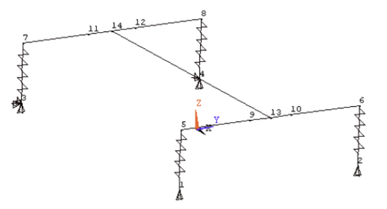
This image depicts a single rigid body for a frame, and four springs representing the suspension. There are now 6 generalised coordinates for the system, describing the position and rotation (I use Euler angles) of the full frame.
However, to write the Lagrangian, we need to write the energy stored in the springs and the kinetic energy of the system in terms of the generalised coordinates. The expressions in this will become absolutely horrible and completely intractable by any human. However, using a symbolic algebra package like SymPy, we can directly write down these equations. This is a mostly uninteresting endeavour, but it can definitely be done! The general strategy for this is to write symbolic expressions for the positions of key tracked points, and then writing expressions for the distances of these points to work out spring lengths and thus energy.

Armed with a symbolic expression of the Lagrangian, we can now generate one equation of motion for each of the generalised coordinates using the Euler-Lagrange equations from before. But how does this allow us to time evolve the system? Let's take a look at the equation from before:
$$\frac{\mathrm{d}}{\mathrm{d}t}\left[\frac{\partial L}{\partial \dot{q_j}}\right]-\frac{\partial L}{\partial q_j}=Q_j^{NC}$$
The first point of action is to deal with the non-conservative generalised forces $Q_j^{NC}$. Recall their definition
$$Q_j^{NC}=\sum _i{\overrightarrow{F_i}}^{NC}\cdot \frac{\partial \overrightarrow{r_i}}{\partial q_j}$$
These forces can represent multiple things in this model, including:

• Aerodynamic forces
• Damper forces
• But most importantly, tire ground forces.

The most efficient way to implement this in the program is to implement this as some set of forces with known direction, but unknown magnitude. Write each non-conservative force as $c_k\widehat{\overrightarrow{F_k}}$, where $c_k$ is the magnitude of the $k$'th non-conservative force and $\widehat{\overrightarrow{F_k}}$ is a unit vector in the direction of the force. $\widehat{\overrightarrow{F_k}}$ does not have to be constant, but for this formulation to work, we need to be able to write $\widehat{\overrightarrow{F_k}}$ symbolically using SymPy.

As an example of this formulation, to represent arbitrary tire-ground forces, declare two non-conservative forces for each tire, one for the longitudinal component and one for the lateral component. If one of our generalised coordinates is the yaw of the car ($\alpha$), then we can write our two $\widehat{\overrightarrow{F_k}}$ as $\hat{\mathbf{i}}\cos \alpha +\hat{\mathbf{j}}\sin \alpha$ and $-\hat{\mathbf{i}}\sin \alpha +\hat{\mathbf{j}}\cos \alpha$.

Now for each $\widehat{\overrightarrow{F_k}}$, if $\overrightarrow{r_k}$ is the position vector of its point of application, then the contribution of this generalised force to the non-conservative generalised force $Q_j^{NC}$ is $c_k\cdot (\widehat{\overrightarrow{F_k}}\cdot \frac{\partial \overrightarrow{r_k}}{\partial q_j})$, and the total generalised force is:
$$Q_j^{NC}=\sum _k{c}_k\cdot (\widehat{\overrightarrow{F_k}}\cdot \frac{\partial \overrightarrow{r_k}}{\partial q_j})$$
We can now write a symbolic expression for each $\widehat{\overrightarrow{F_k}}\cdot \frac{\partial \overrightarrow{r_k}}{\partial q_j}$, and we can express each $Q_j^{NC}$ as a linear combination of these symbolic expressions. Our equation now looks as follows:
$$\frac{\mathrm{d}}{\mathrm{d}t}\left[\frac{\partial L}{\partial \dot{q_j}}\right]-\frac{\partial L}{\partial q_j}=\sum _k{c}_k\cdot (\widehat{\overrightarrow{F_k}}\cdot \frac{\partial \overrightarrow{r_k}}{\partial q_j})$$
It is now time to deal with the left hand side of the expression. Before we proceed though, let's think more about the specific Lagrangian in question for most mechanical systems.
As we established earlier, we can write each $\overrightarrow{r_i}$ as some function of the generalised coordinates, $\overrightarrow{r_i}(\overrightarrow{q})$. We also established that the potential $V$ was only dependent on the generalised coordinates and not the velocities for the above derivation to work. Note that in cases where working with electromagnetic fields, this may not necessarily be true! However, it is true in our case.

Thus, the Lagrangian is
$$\begin{array}{rl}L& =T-V\\ & =\sum _i\frac{1}{2}{m}_i{(\frac{\mathrm{d}}{\mathrm{d}t}(\overrightarrow{r_i}(\overrightarrow{q})))}^2-V(\overrightarrow{q})\\ & =\sum _i\frac{1}{2}{m}_i{\left(\frac{\partial \overrightarrow{r_i}}{\partial \overrightarrow{q}}\dot{\overrightarrow{q}}\right)}^2-V(\overrightarrow{q})\end{array}$$Denote $\frac{\partial \overrightarrow{r_i}}{\partial \overrightarrow{q}}=F_i(\overrightarrow{q})$ The LHS of the equation of motion then becomes
$$\begin{array}{rl}\frac{\mathrm{d}}{\mathrm{d}t}\left[\frac{\partial L}{\partial \dot{\overrightarrow{q}}}\right]-\frac{\partial L}{\partial \overrightarrow{q}}& =\frac{\mathrm{d}}{\mathrm{d}t}\left[\sum _i{m}_i{(F_i(\overrightarrow{q}))}^2\dot{\overrightarrow{q}}\right]-\frac{\partial L}{\partial \overrightarrow{q}}\\ & =[\sum _i{m}_i{(F_i(\overrightarrow{q}))}^2\ddot{\overrightarrow{q}}+\sum _{i}2m_i(F_i(\overrightarrow{q})){\dot{\overrightarrow{q}}}^2]-\frac{\partial L}{\partial \overrightarrow{q}}\end{array}$$
This equation implicitly puts the equations of motion in a vector, to slightly simplify the notation.
The main point of this is to show that for some functions $P(\overrightarrow{q},\dot{\overrightarrow{q}})$ and $Q(\overrightarrow{q},\dot{\overrightarrow{q}})$, the entire LHS can be written as
$$\frac{\mathrm{d}}{\mathrm{d}t}\left[\frac{\partial L}{\partial \dot{\overrightarrow{q}}}\right]-\frac{\partial L}{\partial \overrightarrow{q}}=P(\overrightarrow{q},\dot{\overrightarrow{q}})\ddot{\overrightarrow{q}}+Q(\overrightarrow{q},\dot{\overrightarrow{q}})$$
And for a single equation of motion,
$$\frac{\mathrm{d}}{\mathrm{d}t}\left[\frac{\partial L}{\partial q_j}\right]-\frac{\partial L}{\partial q_j}=P_j(\overrightarrow{q},\dot{\overrightarrow{q}})\cdot \ddot{\overrightarrow{q}}+Q_j(\overrightarrow{q},\dot{\overrightarrow{q}})$$
This seems meaningless, but its consequences are immense. This opens a window into our strategy to time evolve the system: write the motion simply as a first order ODE. If we can somehow compute $\ddot{\overrightarrow{q}}$ from $\overrightarrow{q},\dot{\overrightarrow{q}}$ (or in English, compute "accelerations" of the generalised coordinates given their positions and velocities), then we can put the entire problem into any ODE solver to make progress, as $\frac{\mathrm{d}}{\mathrm{d}t}[\overrightarrow{q},\dot{\overrightarrow{q}}]=[\dot{\overrightarrow{q}},\ddot{\overrightarrow{q}}]$, and the RHS of this expression is now a function of $\overrightarrow{q},\dot{\overrightarrow{q}}$.

So, let's get to it! Each equation of motion is now written as
$$P_j(\overrightarrow{q},\dot{\overrightarrow{q}})\cdot \ddot{\overrightarrow{q}}+Q_j(\overrightarrow{q},\dot{\overrightarrow{q}})=\sum _k{c}_k\cdot (\widehat{\overrightarrow{F_k}}\cdot \frac{\partial \overrightarrow{r_k}}{\partial q_j})$$
We can continue to use our symbolic algebra program to compute $P_j(\overrightarrow{q},\dot{\overrightarrow{q}})$. We do this by computing
$$P_j(\overrightarrow{q},\dot{\overrightarrow{q}})=\frac{\partial }{\partial \ddot{\overrightarrow{q}}}\{\frac{\mathrm{d}}{\mathrm{d}t}\left[\frac{\partial L}{\partial q_j}\right]-\frac{\partial L}{\partial q_j}\}$$
which can be done once again by using SymPy. Once we have computed all $P_j$, we create a symbolic expression called $b_j(\overrightarrow{q},\dot{\overrightarrow{q}})$ containing
$$b_j(\overrightarrow{q},\dot{\overrightarrow{q}})=\sum _k{c}_k\cdot (\widehat{\overrightarrow{F_k}}\cdot \frac{\partial \overrightarrow{r_k}}{\partial q_j})-Q_j(\overrightarrow{q},\dot{\overrightarrow{q}})$$
We can simply do this by substituting all $\ddot{q_j}$ with 0 in the expression for $\frac{\mathrm{d}}{\mathrm{d}t}\left[\frac{\partial L}{\partial q_j}\right]-\frac{\partial L}{\partial q_j}$.
Now each equation of motion is in the form
$$P_j(\overrightarrow{q},\dot{\overrightarrow{q}})\cdot \ddot{\overrightarrow{q}}=b_j(\overrightarrow{q},\dot{\overrightarrow{q}})$$
To be able to solve for $\ddot{\overrightarrow{q}}$, we need to take all of the equations of motions together. We do this by stacking each of the expressions for $P_j$ into a matrix, ${\mathbf{P}}_{\mathbf{j}}(\overrightarrow{q},\dot{\overrightarrow{q}})$ and all of the expressions for $b_j(\overrightarrow{q},\dot{\overrightarrow{q}})$ into a vector $\overrightarrow{b}(\overrightarrow{q},\dot{\overrightarrow{q}})$.
This then creates the overall equation
$${\mathbf{P}}_{\mathbf{j}}(\overrightarrow{q},\dot{\overrightarrow{q}})\cdot \ddot{\overrightarrow{q}}=b_j(\overrightarrow{q},\dot{\overrightarrow{q}})$$
But this is now just an equation of the form $\mathbf{A}\overrightarrow{x}=\overrightarrow{b}$, where $\mathbf{A}$ and $\overrightarrow{b}$ are functions of $\overrightarrow{q},\dot{\overrightarrow{q}}$. We can use any linear system solver to find $\overrightarrow{x}$, or in this case $\ddot{\overrightarrow{q}}$.

Now to compute $\ddot{\overrightarrow{q}}$ given numerical values for $\overrightarrow{q},\dot{\overrightarrow{q}}$, we simply substitute $\overrightarrow{q},\dot{\overrightarrow{q}}$ into ${\mathbf{P}}_{\mathbf{j}}(\overrightarrow{q},\dot{\overrightarrow{q}})$ and $\overrightarrow{b}(\overrightarrow{q},\dot{\overrightarrow{q}})$ Note that $\overrightarrow{b}$ also depends on the magnitude of the non-conservative forces $c_k$. We can then simply solve the resulting linear system of equations to obtain $\ddot{\overrightarrow{q}}$.

To summarise, here is how the overall time evolution of the system works:

• At each time step:
  • Take the current values of $\overrightarrow{q}$ and $\dot{\overrightarrow{q}}$ (the values and first time derivatives of the generalised coordinates)
  • Use some external function to compute the magnitudes of all of the non-conservative forces $c_k$ from the current values and time derivatives of the generalised coordinates.
    • In the case of the car system, this will involve finding the slip angles of all of the wheels and feeding them into some tire model to calculate tire forces, or finding the aerodynamic force from the velocity of the car.
  • Calculate ${\mathbf{P}}_{\mathbf{j}}(\overrightarrow{q},\dot{\overrightarrow{q}})$ and $\overrightarrow{b}(\overrightarrow{q},\dot{\overrightarrow{q}})$, and use the above procedure to find the second derivatives of the generalised coordinates, $\ddot{\overrightarrow{q}}$.
  • Use a standard ODE solution method (e.g. RK45, but in practice I use SciPy built-ins like solve_ivp) to find the values of $\overrightarrow{q}$ and $\dot{\overrightarrow{q}}$ at the next timestep.
    • To elaborate on this, we create the state vector $\overrightarrow{s}=[\overrightarrow{q};\dot{\overrightarrow{q}}]$. All the steps above allow us to write $\dot{\overrightarrow{s}}$ as a function of $\overrightarrow{s}$ i.e. creating a first order ODE to be solved using an IVP solver.

Closing remarks

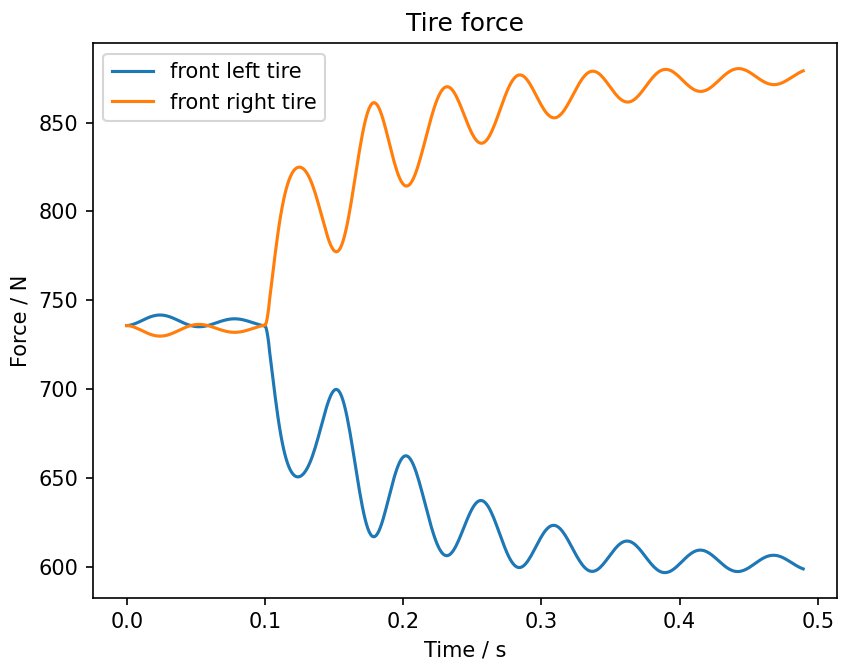
The power of this method is in the sheer complexity that a single model can encapsulate. We no longer have to model cars with simple bicycle models with steady state formulae; we have a generalised method to evolve models as complex as they get. The use of generalised coordinates also allows us to directly track values of interest, such as the yaw rate of the car or the roll of the car. The use of symbolic algebra expressions allow other values of interest (e.g. shock length, tire normal forces) to be easily computed on top of this. To showcase the power of this model, here is a graph showing load transfer as a driver enters a turn following a step steering input:

And here is a video of a simulated car drifting!

Room for improvement

No project is truly done without thinking about where you can go next!

• The simulation speed is quite slow at the moment. Straights run fine, but cornering is up to 10x slower than real time
  • This makes lap time simulation quite difficult. I have an entire layer on top of this to somehow precalculate cornering speeds to allow single laps to be run in reasonable amounts of time.
  • This could almost definitely be greatly alleviated simply by porting code to C++. At the moment, I am using Numba compilation to speed up function evaluation, but to use SciPy's IVP solver, the data is brought back into Python at each time step for further processing
• It is somewhat difficult to model nonlinear suspension into this model: a lot of suspension is designed with a progressive motion ratio, which cannot be simply modelled in this system
  • Time permitting, we will look into potentially constructing new potential functions to account for this.
• Some problems do become harder
  • Solving for steady state corners, for example, has proven to be somewhat difficult
    • This may be true because steady state corners may not exist due to modelled dissipation. However, it should still be possible to find "close enough" solutions.
• There are kind of "follow-on" problems on how to utilise the power of this model. For example, how would corners best be modelled? It is now a new challenge to find the optimal driver inputs / racing line to simulate for the car when going around a circuit.

But overall, I am super happy with model and its power, and I can't wait to see where the project goes next!