Visualising audio on an LED strip with Python and an Arduino

For a while, I’ve wanted to use my WS2812B LED light strips to visualise music, and today, I created a program to do just that.
If you are impatient and would just like to see this in action, scroll to the bottom of the article for videos.

Approaching the problem

At first, I decided that the obvious way to go about this would be using a Fourier transform. This is a transform that could decompose a wave (like the sound being played) into its component frequencies. That way, if something with a low frequency and a high frequency was being played, I would be able to decompose them into these components. In addition, I would also be able to spot a changing frequency, like a melody. I fiddled with this idea for a bit, and decided to make a spectrogram.

For all of the following examples in this article, I’m using the first 10 seconds of “Toss A Coin To Your Witcher”.
A spectrogram performs a Fourier transform locally at many points to determine the intensity of individual frequencies in the wave. It then displays this with time on the x-axis and frequency on the y-axis, with the colour at each point representing intensity.

With matplotlib and scipy, this code for this is very simple.

import matplotlib.pyplot as plt
from scipy import signal
from scipy.io import wavfile

FS, data = wavfile.read('wavs/witchershort.wav')
plt.specgram(data, Fs=FS, NFFT=256, noverlap=0, scale='dB')  # plot
plt.show()

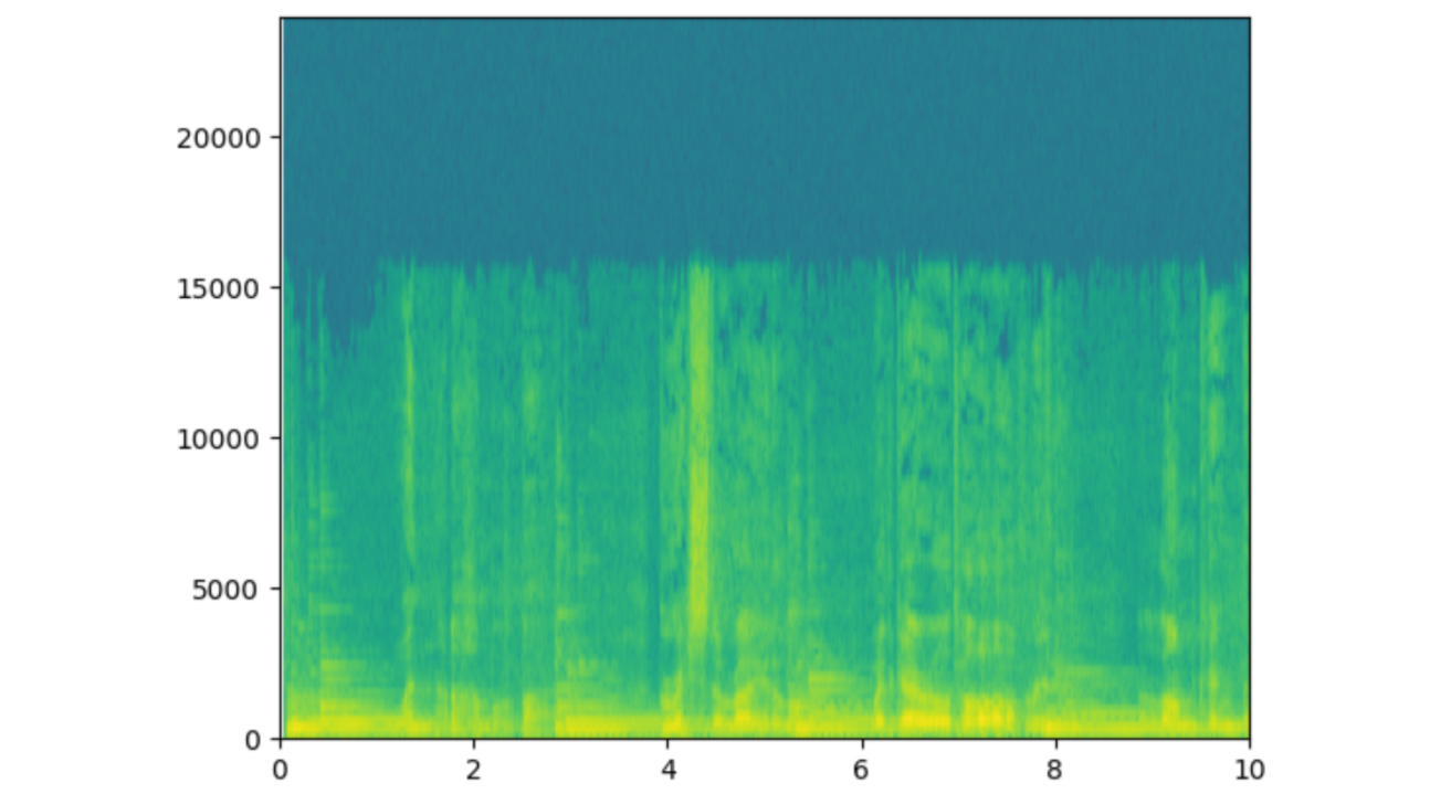
Here is the spectrogram of the audio:

We can clearly see that this is linked to the audio - somehow? It’s not entirely clear what’s going here either though.
Notice how high the frequencies are as well: the y-axis is frequency in Hz, and 5000 is already a decently high frequency. Most musical notes are much lower frequencies, in the 20 - 1000Hz range. If we zoom in, all we see is a garbled set of rectangles.

Part of the problem is that the Fourier transform inherently has difficulties detecting low frequencies. If we perform the Fourier transform over a 1/60th of a second slice of time (or 0.0167 seconds), it’ll be difficult to detect frequencies as low as, say, 40Hz, as a single wavelength of this frequency takes 1/40 = 0.0250 seconds to pass. In addition, small changes in the lower frequencies are proportionally much larger and much easier to detect with the human ear - it’s way easier to tell the difference between 40 and 60Hz than it is between 4000 and 4020Hz.

I also wanted to work with a much simpler method, so I turned to directly looking at the intensity of the audio.

Working with the amplitude of the audio

WAV files contain the intensity of audio at thousands of different points in time. There can be around 48,000 of these samples in a single second, even in lower quality audio. A negative intensity corresponds to a lower-than-atmospheric pressure in air (because sound is just air pressure moving as a wave).

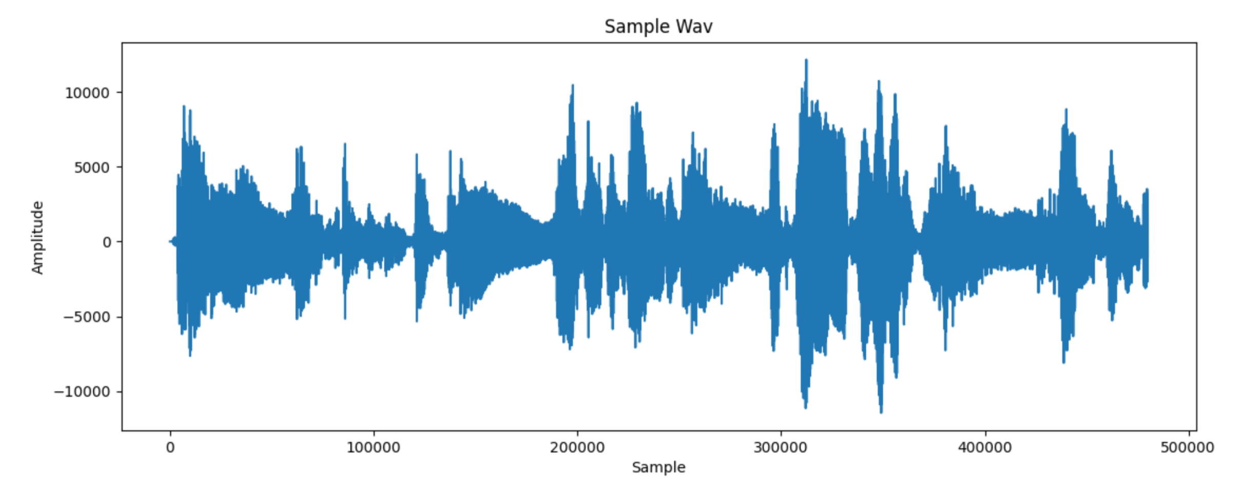
Plotting all of these out, we get a familiar sound-wave-esque curve.

However, notice that on the x-axis there are nearly 5 million samples in the first 10 seconds, which seems pretty excessive for a visualisation that realistically only needs to update 60 times a second.

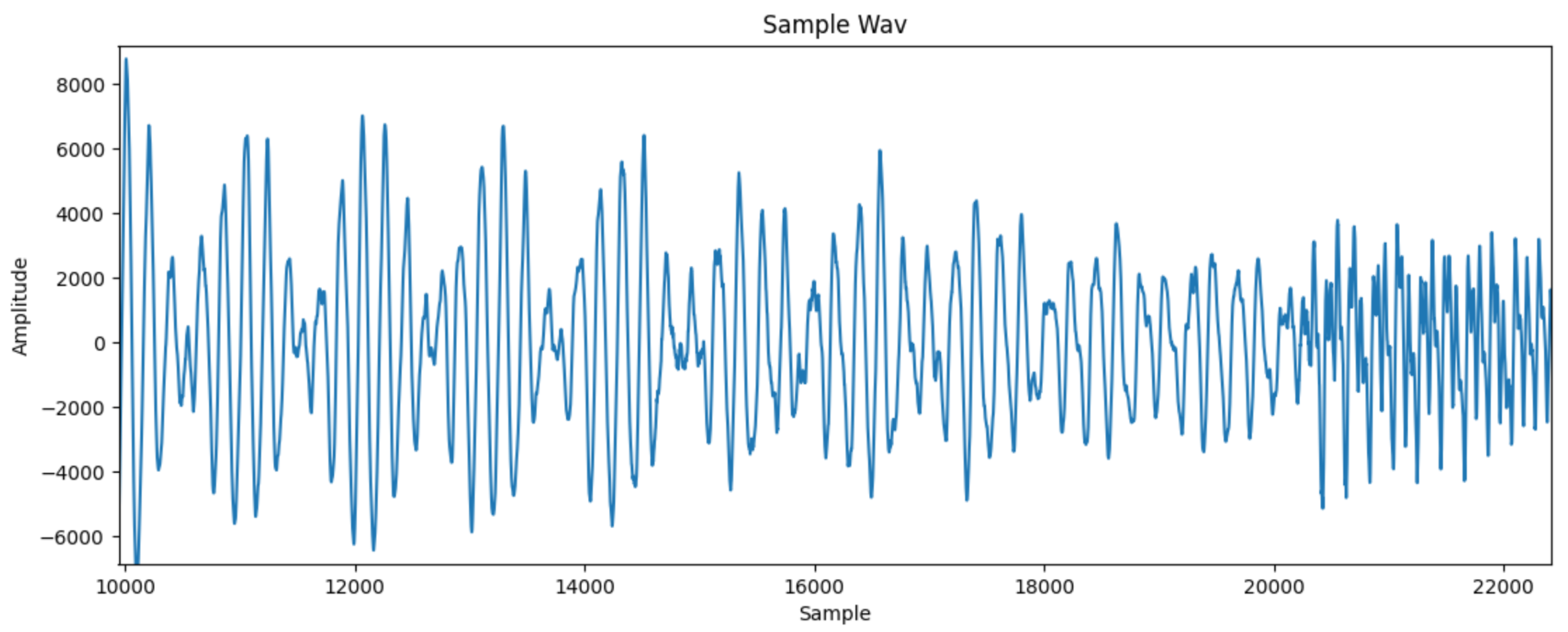
Zooming in, we also come across our first problem.

This is a wave that moves up and down, not clearly corresponding to an intensity. We want to somehow smooth out this curve, and lose lots of the sample data while doing so.

A simple way to get started is to group samples into batches that cover 1/60th of a second. For example, if a file had 48000 samples per second, we would want 48000 / 60 = 800 samples in each batch. In each batch, we could just sum all of the samples, but the negative values would mostly cancel out the positive values. To fix this, I only sum the positive values when summing over a sample. To prevent the sums from being too large, I also divide them by the number of samples, to essentially give an average of all positive samples in each 1/60th of a second.

To do this, I used this code:

smoothing_range = sample_rate / 60
frames = math.ceil(len(audio) / smoothing_range)
maxima = np.zeros((frames,), dtype=float)

step = math.floor(sample_rate / 600)
for x in range(0, len(audio)):
    sample = audio[x]
    # calculate what frame we are in
    frame = math.floor(x / smoothing_range)
    if (sample > 0):
        maxima[frame] += (sample / smoothing_range)

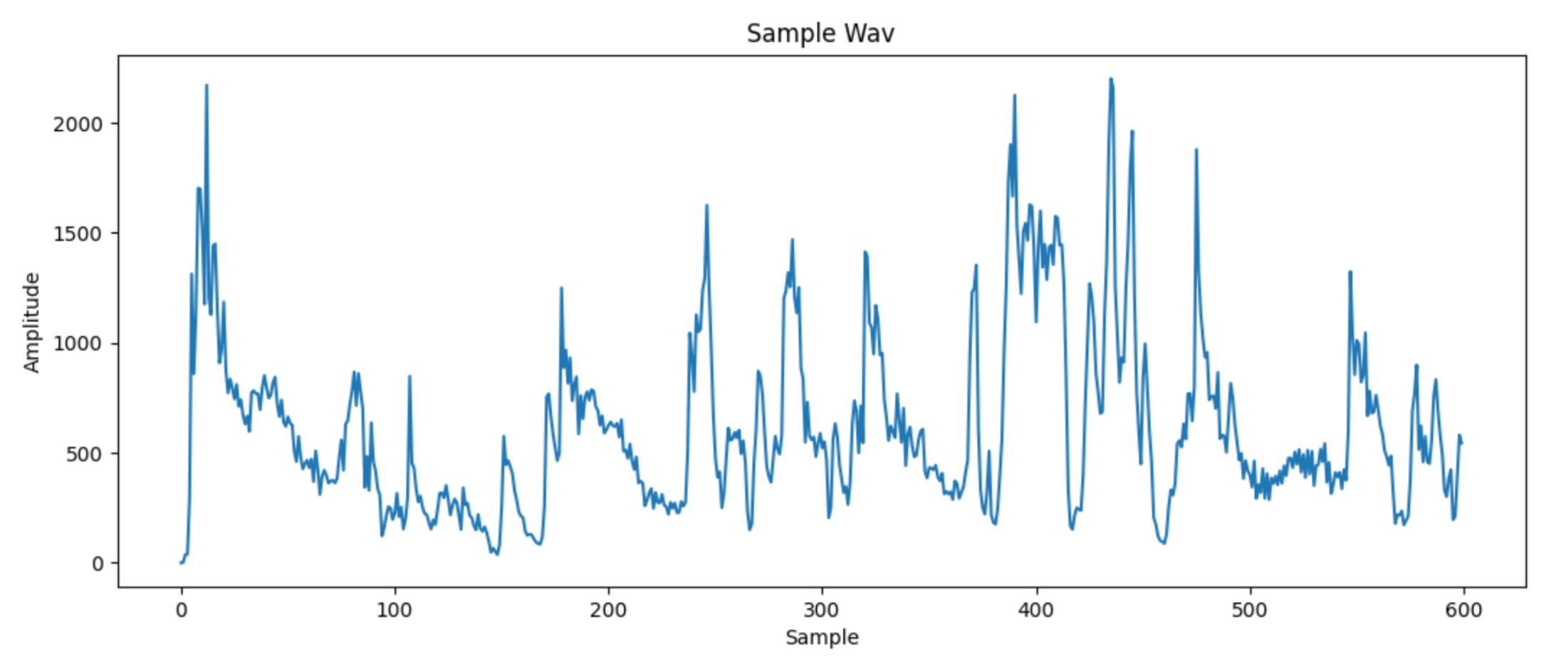
This leaves us with this plot:

This is looking much more manageable, but still seems quite rough. We have also reduced the space to 600 data points, one for each 1/60th of a second. I’ll be now referring to each of these as frames. To smoothen the curve out, I take a local average of 10 frames on each frame. This means that sudden changes will be attenuated.

This can be done by simply looping through all the frames and then looping through their surroundings. While this isn’t efficient at all, there are few enough frames that it isn’t a problem.

smooth_size = 5
maxima_smoothed = np.zeros((frames,), dtype=float)
for x in range(frames):
    range_min = max(x - smooth_size, 0)
    range_max = min(x + smooth_size, frames)
    for y in range(range_min, range_max):
        maxima_smoothed[x] += maxima[y]
    maxima_smoothed[x] /= (range_max - range_min)

Now the plot looks like this:

This is now reaching the point where it’s actually possible to make out what parts of the song are being shown in the wave, so I’ve labelled them on the image above.

This is already pretty good for a visualisation. Many audio visualisation have sufficed with just displaying the intensity of the audio being played.
However, I wanted to try and take this to the next step.

Detecting peaks

Imagine I was tapping out a song. Now my “display” is no longer continuous - instead, I will simply “tap” at different points in time.

To try and “detect” these “tapping points”, I would move on to looking at local maxima of the intensity, which I call peaks. As we can see above, most words come at local points of intensity, and it makes sense that we could do something different at these points.

First, however, I need a way to detect them. I have implemented a very simple peak detection algorithm. This works by looking 10 frames to the left and right of the current frame that we are looking at. I will call these the left frame and right frame.
If the intensity of the current frame is not greater than that of the left or right frames, then this is obviously not a peak (or quite a small one).
Next, we need a way to say “how peaky is a peak?”. We could obviously look at the differences of the left and right frame from the current frame, but we don’t want large peaks to be emphasized too much more than the smaller peaks. As a small measure to combat this, I simply square rooted these differences before averaging them. I call the value that I get from this process the peak coefficient of each frame.

I then scale all the peak coefficients by 100 to make them more similar in size to the frame intensities themselves.
Experimentation shows that it is reasonable to eliminate the peak coefficients with value less than 1500 after this scaling.

The code to get the peak coefficients is below:

search_size = 10
peakcoeff = np.zeros((frames,), dtype=float)
for x in range(frames):
    range_min = maxima_smoothed[max(x - search_size, 0)]
    currvalue = maxima_smoothed[x]
    range_max = maxima_smoothed[min(x + search_size, frames - 1)]

    if (range_min < currvalue) and (range_max < currvalue):
        diff1 = currvalue - range_min
        diff2 = currvalue - range_max
        peakcoeff[x] = (math.sqrt(diff1) + math.sqrt(diff2)) / 2
    else:
        peakcoeff[x] = 0
    peakcoeff[x] *= 100
    if (peakcoeff[x] < 1500):
        peakcoeff[x] = 0

This then leaves me with this graph, where the orange line is the peak coefficient at each point.

I was now pretty happy with the processing I had done. I now needed to turn this into an Arduino visualisation.
I decided that I was going to stream the data over Serial to the Arduino, while playing the audio at the same time on my machine.
To make these run concurrently, I had to use asynchronous programming. To do this, I used the asyncio library.
First, I create an async function that is precisely timed to send data every 1/60th of a second. To prevent it from falling out of sync, I don’t just wait for 1/60th of a second every time I send my data. Instead, I store a start time, and every time I go through the loop, I make sure to wait until the next integer multiple of 1/60 = 0.0167 seconds before rerunning the loop.

Before this though, I needed to think about what format my Serial communication would take. Every frame, I need to send the intensity and peak coefficient of the current frame. While I could send the accurate value (which is in the range of 1000s), I scale both of these values down to under 255 so that they can fit into single bytes. I then create a four byte packet, with the byte 254 indicating the start, then the next 2 bytes containing peak coefficient and intensity information, and finally the byte 253 to indicate the end of the packet.

I use asyncio.gather to start this communication at the same time as playing the sound locally on the PC.

async def main():
    global peakcoeff, maxima_smoothed, frames, ser
    async def printvalues():
        starttime = time.time()
        for x in range(frames):
            await asyncio.sleep((1 / 60) - ((time.time() - starttime) % (1 / 60)))
            bytes_data = [254, min(math.floor(peakcoeff[x] / 50), 255), min(255, math.floor(maxima_smoothed[x] / 50)), 253]
            ser.write(bytes(bytes_data))
            # print(peakcoeff[x], maxima_smoothed[x])

    @async_wrap
    def play():
        playsound(audio_path)
    
    await asyncio.gather(play(), printvalues())
    ser.close()

asyncio.run(main())

Controlling the LED strip with an Arduino

To make sure that the Arduino could get as much data as possible, I set its baud rate to 115200, meaning that it can transfer 115200 bits (or about 15kB) every second.

The Arduino can very easily be interfaced with the WS2812B LED light strip. It can share 5V and GND directly with the Arduino, and only a single current limiting resistor is required on the data pin. After this, the Adafruit Neopixel library does all the work, allowing us to set the colour of individual LEDs.

Now I needed to think of some simple, yet aesthetically pleasing way to display the information.
I decided to have a different number of the bottom LEDs light up depending on the intensity of the audio, and have the top LEDs light up on a peak. The LEDs that would light up on a peak would “waterfall” down with time.
Finally, to add another dimension to the visualisation, I also decided to change the hue of all the colours depending on intensity, with cool blues for quiet songs and loud oranges and yellows for louder sections.

I bunched this together into this quick program:

#include <Adafruit_NeoPixel.h>
#ifdef __AVR__
 #include <avr/power.h> // Required for 16 MHz Adafruit Trinket
#endif

// Which pin on the Arduino is connected to the NeoPixels?
// On a Trinket or Gemma we suggest changing this to 1:
#define LED_PIN    6

// How many NeoPixels are attached to the Arduino?
#define LED_COUNT 60

// Declare our NeoPixel strip object:
Adafruit_NeoPixel strip(LED_COUNT, LED_PIN, NEO_GRB + NEO_KHZ800);

int bytesin[4];
int frameparity = 0;
int lit[LED_COUNT];
int pointer = 0;
bool prevthresh = false;

void setup() {
  // put your setup code here, to run once:
    strip.begin();           // INITIALIZE NeoPixel strip object (REQUIRED)
  strip.show();            // Turn OFF all pixels ASAP
  strip.setBrightness(50); // Set BRIGHTNESS to about 1/5 (max = 255)
  Serial.begin(115200);
  pinMode(13, OUTPUT);
  digitalWrite(13, LOW);
}

void loop() {
  // put your main code here, to run repeatedly:
  if (Serial.available() > 0) {
    // read the incoming byte:
    int incomingByte = Serial.read();
    if (incomingByte == 254) {
      pointer = 0;
    }
    else if (incomingByte == 253) {
      if (pointer == 3) {
        // rotate
        for (int i = LED_COUNT - 1; i >= 0; i--) {
          lit[i] = lit[i - 1];
        }
        lit[0] = false;
        if (bytesin[1] > 0) {
          lit[0] = bytesin[1];
          prevthresh = true;
          digitalWrite(13, HIGH);
        }
        else {
          prevthresh = false;
          digitalWrite(13, LOW);
        }
        
        for (int i = 0; i < LED_COUNT; i++) {
          if (lit[i]) {
            strip.setPixelColor(60 - i, strip.ColorHSV(21845 + (bytesin[2] * 250), 255, (255 - bytesin[2])));
          }
          else {
            strip.setPixelColor(60 - i, 0, 0, 0);
          }

          if ((60 - i) < (bytesin[2] / 3)) {
            strip.setPixelColor(60 - i, strip.ColorHSV(53000 + (bytesin[2] * 250)));
          }

          if ((60 - i) == (bytesin[2] / 3)) {
            strip.setPixelColor(60 - i, 255, 255, 255);
          }
        }
        strip.show();                          //  Update strip to match
      }
    }
    if (pointer < 4) {
      bytesin[pointer] = incomingByte;
    }
    pointer += 1;
  }
}

Streamlining the full process

Up until now, I had only been working with raw audio files. I used the youtube-dl package to allow me to input a YouTube URL. I then downloaded the mp4 of the video from youtube, extracted a .wav audio file using ffmpeg, and then ran the whole process.

The final code for my audio processor is below:

from scipy.io.wavfile import read
from scipy.ndimage.filters import gaussian_filter1d
import matplotlib.pyplot as plt
import math
import numpy as np
from repeated_timer import RepeatedTimer
from playsound import playsound
import asyncio
from functools import wraps, partial
import time
import serial

# read audio samples
import os
import subprocess
import youtube_dl

if os.path.exists("audio.wav"):
    os.remove("audio.wav")

import glob
import os

def delete_files(path, pattern):
    for f in glob.iglob(os.path.join(path, pattern)):
        try:
            os.remove(f)
        except OSError as exc:
            print(exc)

delete_files("", "video.*")

vid_url = input("Enter a youtube URL: ")
ydl_opts = {
    'outtmpl': "video"
}
with youtube_dl.YoutubeDL(ydl_opts) as ydl:
    ydl.download([vid_url])

video_file = None
for f in glob.iglob(os.path.join("", "video.*")):
    video_file = f

subprocess.call('ffmpeg -i ' + video_file + ' -ac 1 audio.wav', shell=True)
print("Converted file to WAV")

audio_path = "audio.wav"
sample_rate, audio = read(audio_path)
ser = serial.Serial('COM9', 115200)
print("Opened connection to Arduino")

smoothing_range = sample_rate / 60
frames = math.ceil(len(audio) / smoothing_range)
maxima = np.zeros((frames,), dtype=float)

step = math.floor(sample_rate / 600)
for x in range(0, len(audio)):
    sample = audio[x]
    # calculate what frame we are in
    frame = math.floor(x / smoothing_range)
    if (sample > 0):
        maxima[frame] += (sample / smoothing_range)

print("Finished initial WAV process")
# now do local averaging
smooth_size = 5
maxima_smoothed = np.zeros((frames,), dtype=float)
for x in range(frames):
    range_min = max(x - smooth_size, 0)
    range_max = min(x + smooth_size, frames)
    for y in range(range_min, range_max):
        maxima_smoothed[x] += maxima[y]
    maxima_smoothed[x] /= (range_max - range_min)

# next, look for local peaks
search_size = 10
peakcoeff = np.zeros((frames,), dtype=float)
for x in range(frames):
    range_min = maxima_smoothed[max(x - search_size, 0)]
    currvalue = maxima_smoothed[x]
    range_max = maxima_smoothed[min(x + search_size, frames - 1)]

    if (range_min < currvalue) and (range_max < currvalue):
        diff1 = currvalue - range_min
        diff2 = currvalue - range_max
        peakcoeff[x] = (math.sqrt(diff1) + math.sqrt(diff2)) / 2
    else:
        peakcoeff[x] = 0
    peakcoeff[x] *= 100
    if (peakcoeff[x] < 1500):
        peakcoeff[x] = 0

print("Finished full processing, playing...")

def async_wrap(func):
    @wraps(func)
    async def run(*args, loop=None, executor=None, **kwargs):
        if loop is None:
            loop = asyncio.get_event_loop()
        pfunc = partial(func, *args, **kwargs)
        return await loop.run_in_executor(executor, pfunc)
    return run
# finally, quantise the peaks
async def main():
    global peakcoeff, maxima_smoothed, frames, ser
    async def printvalues():
        starttime = time.time()
        for x in range(frames):
            await asyncio.sleep((1 / 60) - ((time.time() - starttime) % (1 / 60)))
            bytes_data = [254, min(math.floor(peakcoeff[x] / 50), 255), min(255, math.floor(maxima_smoothed[x] / 50)), 253]
            ser.write(bytes(bytes_data))
            # print(peakcoeff[x], maxima_smoothed[x])

    @async_wrap
    def play():
        playsound(audio_path)
    
    await asyncio.gather(play(), printvalues())
    ser.close()
    # playsound(audio_path)
asyncio.run(main())

The final result!

(I hope you didn’t just skip here…)
I taped my LED strip and Arduino to my wall (the image in the thumbnail) and recorded it playing some songs.

Currently, I haven't properly added support for YouTube embeds. You can watch them in small on here or open them in other tabs to see them in full size.

Toss A Coin To Your Witcher - this song worked decently, but not amazingly.

Dizzee Rascal - Fix Up, Look Sharp - this song worked very well, as it had clear intense points for peaks and large, sudden changes in amplitude

Raccy - Through Money - this song also worked well for the same reasons.

He-Man - What’s Up - this song didn’t work as well, as my algorithm was unable to consistently detect the smaller and quicker changes in amplitude.