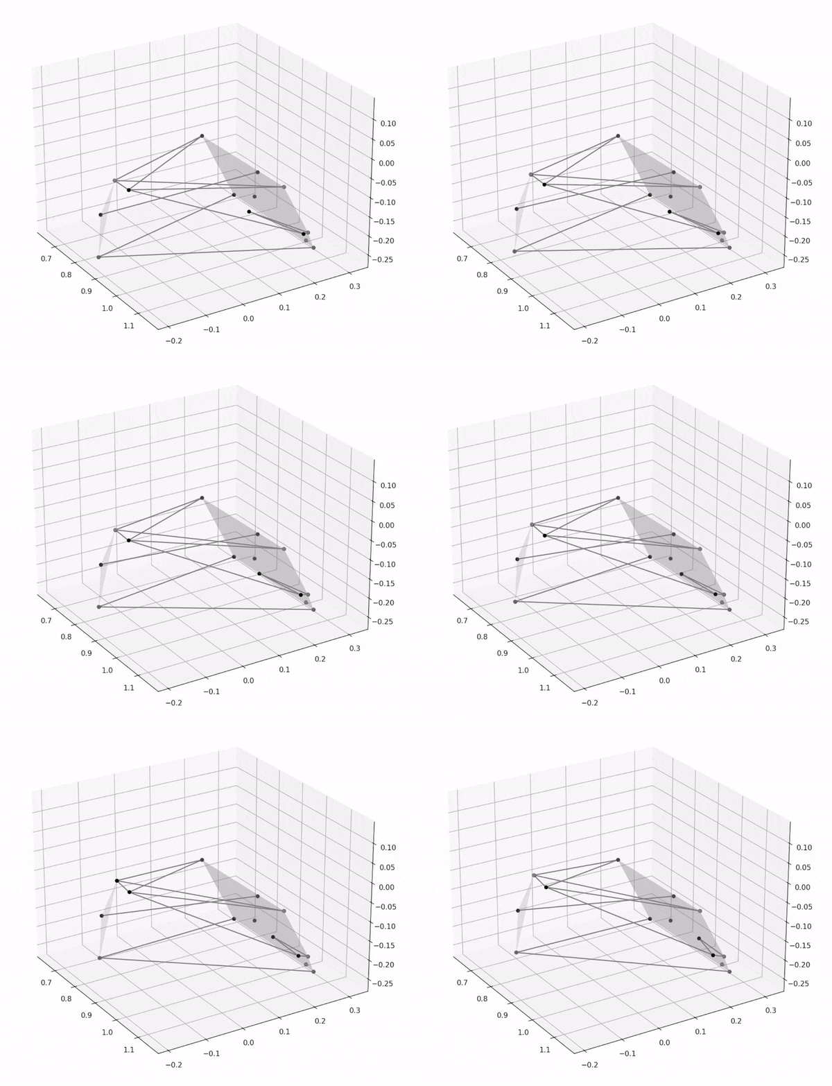
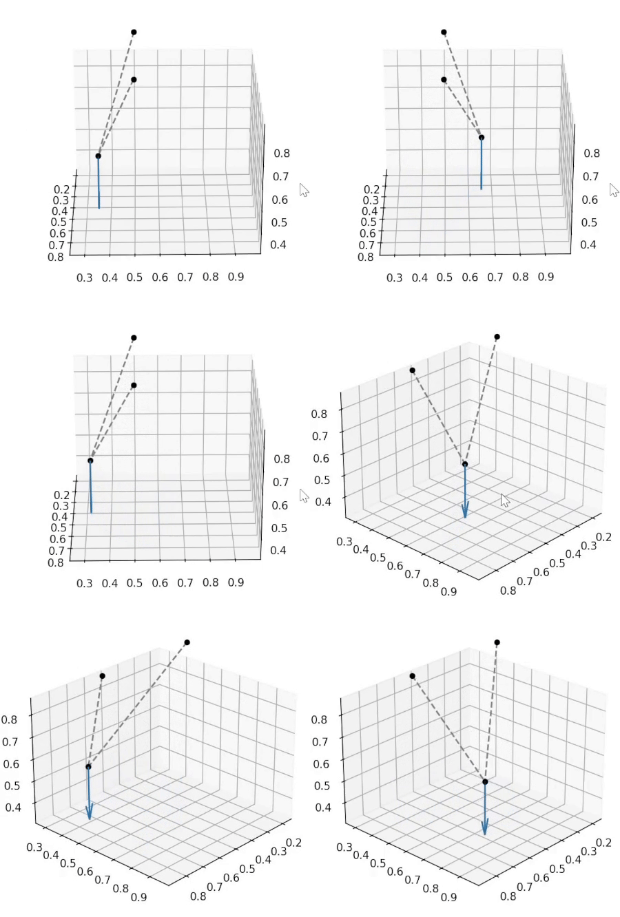
Recently, I've been working on a multibody dynamics simulation, which is a problem that I have had an immense amount of fun tackling recently. I initially wanted to do this to create a dynamics simulation for my Formula Student team, but the simulation is very generalizable to a variety of models and load cases. As far as I know, this method is novel and might be interesting to others. (I am quite proud of it :) )

More impressive is how easy it is to make different models in this system. The right simulation can be generated with just the following python code:

system = ma.System()
origin = system.add_point("originpoint", np.array([[0.25], [0.5], [1]]), fixed=True)
origin2 = system.add_point("originpoint2", np.array([[0.75], [0.5], [1]]), fixed=True)
free_point = system.add_point("freepoint", np.array([[0.65], [0.7], [0.5]]), fixed=False, mass=1)

motion_analysis = ma.MotionAnalysis(system)
motion_analysis.add_fixed_force(free_point, np.array([[0], [0], [-1]])) # gravity
motion_analysis.add_spring_damper(origin, free_point, k=8, b=0, natural_len=0.5)
motion_analysis.add_spring_damper(origin2, free_point, k=8, b=0, natural_len=0.5)

timesteps = 700
res = motion_analysis.simulate(dt=0.02, timesteps)

fig = plt.figure()
ax = fig.add_subplot(projection='3d')
ax.axis('equal')
anim = motion_analysis.animate_scene(res, fig, ax)

What is the goal?

In any design project, it is a good idea to start with some goals. I wanted to be able to:

1. Design a system out of a set of simple primitives: perhaps some points, some rigid links, a few springs and dampers, and maybe some rigid bodies

2. For a given system, identify its degrees of freedom: identify how the system can be perturbed without affecting any of the constraints

3. Apply forces to the system and identify how the system responds to them over time.

4. Potentially, evaluate the constraint forces imposed by the constraints on the system. For an example, consider a ball in a gravitational field rolling on a table. The problem can be simplified by restricting the ball's motion to the xy plane and assuming the z position of the ball is fixed. The constraint force in this case is the normal force from the table on the ball.

How do we describe the system?

It is relatively easy to describe a system in words. I can say "imagine a mass connected to the origin by a 1m long rigid link" and you immediately know what I am talking about. It is still doable to describe a system in software as a set of points and links, but describing a system in a way usable for computation takes some more thought. From Lagrangian and Hamiltonian mechanics, we borrow the idea of a state vector. The state vector is some function \(\vec{q}(t)\) that describes all of the coordinates relevant to describing the system over time. For example, for a system made out of two points free in 3D space, we can define a state vector with 6 elements, the first three describing the x, y, z coordinates of the first point and the next three describing the x, y, z coordinates of the second point. 

So far, we have really not done anything very exciting. It then becomes slightly more difficult to describe the constraints on the system. For exemplary purposes, let's limit out focus to two very basic constraints: fixed points and rigid links. Both of these are holonomic constraints, which are the only ones we will tackle in this article.

Holonomic constraints can easily be written in the form of what I have been calling constraint equations, which are some function of the coordinates that are required to be zero throughout the motion. In other words, they are functions \(f\) such that \(f(\vec{q}(t)) = 0\) for all time t. This is best illustrated with an example.

Consider a point fixed at the origin and a second point fixed to always remain one meter away by a rigid link. Let the state vector \(\vec{q}(t)\) be defined such that \(q_1, q_2, q_3\) are the x, y, and z coordinates of the origin and \(q_4, q_5, q_6\) be the x, y, z coordinates of the free point. We can then write the following constraint equations. First, ensure that the origin point remains at, well, the origin:

\[\begin{gather*} q_1 = 0 \\ q_2 = 0 \\ q_3 = 0 \end{gather*} \]

Next, ensure that the distance between the points is always 1:

\[(q_1 - q_4)^2 + (q_2 - q_5)^2 + (q_3 - q_6)^2 - 1^2 = 0\]

These constraints are quite simple (in fact, there is a good argument for the fixed origin point to not even be included in the state vector, and this is an optimisation that can be made in the future), but they are easily extensible to a variety of situations. For example, we can force the vectors between two points to be perpendicular by ensuring that their dot product is zero.

How do we represent rigid bodies?

This is a quick section on how rigid bodies can be represented in this framework. As we all know, a necessary requirement for rigid bodies is that the distance between any pair of points is constant throughout the motion. A naive idea is to simply link every pair of points in a rigid body, but this will take \(\binom{n}{2}\) links for a rigid body with n points, which is of order \(n^2\). To simplify this problem, we can think about degrees of freedom. n points free in space will normally have \(3n\) degrees of freedom (one for each translational degree of freedom), but a rigid body will only have 6 (3 translational, 3 rotational). This suggests that there are \(3n - 6\) constraints required to take a set of points to a rigid body.

It turns out that that this can be accomplished by connecting just three points to each other and those three points to every other point, which is \(3 + 3(n - 3) = 3n - 6\) constraints as desired. In words, what this is actually doing is picking three points and forming a tetrahedron with every single other free point. The 6 edges of a tetrahedron are sufficient to describe a rigid body, and in this setup the rigid body ends up being represented by multiple tetrahedra with a shared base. This reduces the number of links required from \(O(n^2)\) to \(O(n)\), a massive speedup that will be even more important in the future.

How do we find the degrees of freedom?

This is so far still quite standard procedure, but this is now the first of a few exciting ideas in this project.

We begin by realizing that a degree of freedom is some direction \(\delta \vec{q}\) such that the system state vector can be moved to \(\vec{q} + \delta \vec{q}\) while satisfying all constraints. This "direction" physically describes a small perturbation in the coordinates describing the system. But how do we find these directions?

One way to think about this is to imagine the vector \(\vec{q}\) existing in some d-dimensional space. However, the set of vectors that meet the constraints is some smaller surface existing within this space. To define this surface, we create the vectorial constraint function \(\vec{f}(\vec{q})\). \(\vec{f}\) simply has one component for each value of each constraint function at the given system state \(\vec{q}\). For the previous example of one free point rigidly linked to a fixed point, \(\vec{f}\) would be:

\[\begin{pmatrix} q_1 \\q_2 \\q_3 \\(q_1 - q_4)^2 + (q_2 - q_5)^2 + (q_3 - q_6)^2 - 1^2\end{pmatrix}\]

The surface is then defined with \(\vec{f}(\vec{q}) = 0\).

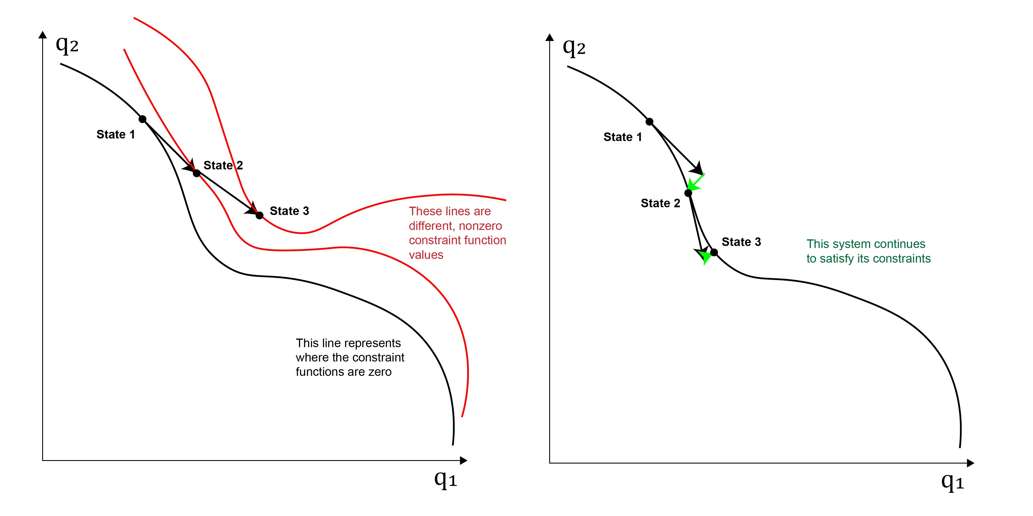
To remain on the surface, the degree of freedom direction \(\delta \vec{q}\) must be tangential to the surface, as otherwise the values of the constraint functions will change. The image below illustrates this idea:

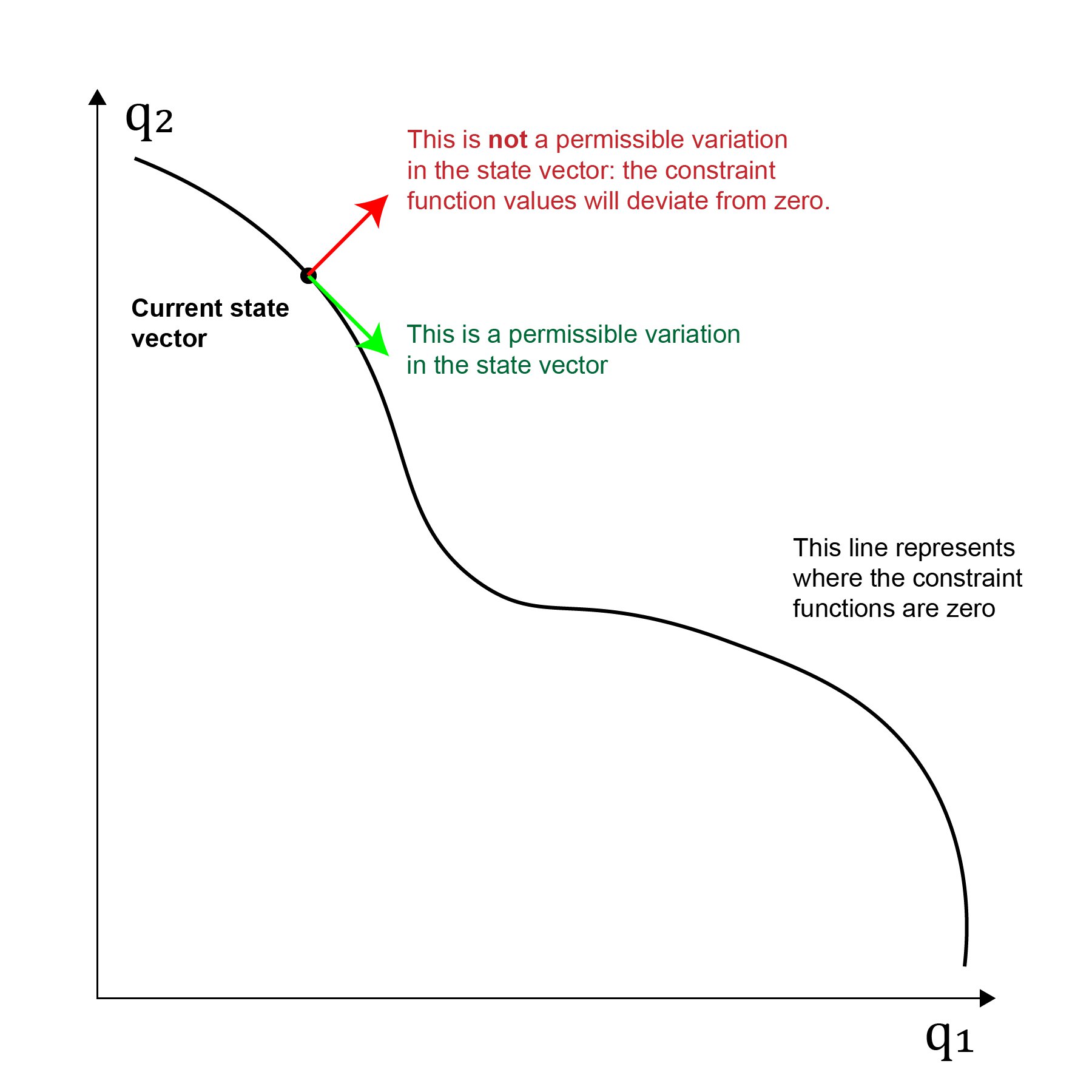
To find these tangential directions, we work more closely with \(\vec{f}\), which simply has one component for each value of the constraint function at the given system state \(\vec{q}\). We can then evaluate the Jacobian matrix \(\frac{\text{d} \vec{f}}{\text{d} \vec{q}}\) \(\def\od#1#2{{\frac{\d #1}{\d #2}}} \def\d{{\text{d}}}\):

\[\od{\vec{f}}{\vec{q}} = \begin{pmatrix}\od{f_1}{q_1} & \od{f_1}{q_2} & \dots & \od{f_1}{q_d} \\ \od{f_2}{q_1} & \od{f_2}{q_2} & \dots & \od{f_2}{q_d} \\ \vdots & & \ddots & \\\od{f_n}{q_1} & \od{f_n}{q_2} & \dots & \od{f_n}{q_d} \end{pmatrix} \]

Now, we can verify steps \(\delta \vec{q}\) as they will satisfy \(\od{\vec{f}}{\vec{q}} \times (\delta \vec{q}) = 0\), i.e. the variation in q does not affect the constraint functions. We have reduced the degrees of freedom problem to finding the right nullspace of a matrix! Even better news is that this matrix is quite easy to evaluate for the fixed point and rigid link constraints as these turn out to have quite simple derivatives, speeding up computation time.

We could attempt to find this nullspace by using standard methods such putting it into reduced row echelon form. However, we are working in the real world with floating point inaccuracies, and it is very possible for some vectors to quickly "fall out" of the nullspace with some errors in the matrix. To overcome this, we use the powerful singular value decomposition of a matrix. This decomposes any matrix A into the form \(USV^*\), where S is a diagonal matrix and V is orthogonal. The nullspace is then described by the columns of V that correspond to 0 entries on the diagonal of S. Most importantly, SVD is stable to perturbations in the input matrix, and so we can simply apply some tolerance to the diagonal entries of S e.g. treat all diagonal entries of S with a value of magnitude less than 0.0000001 as corresponding to degrees of freedom.

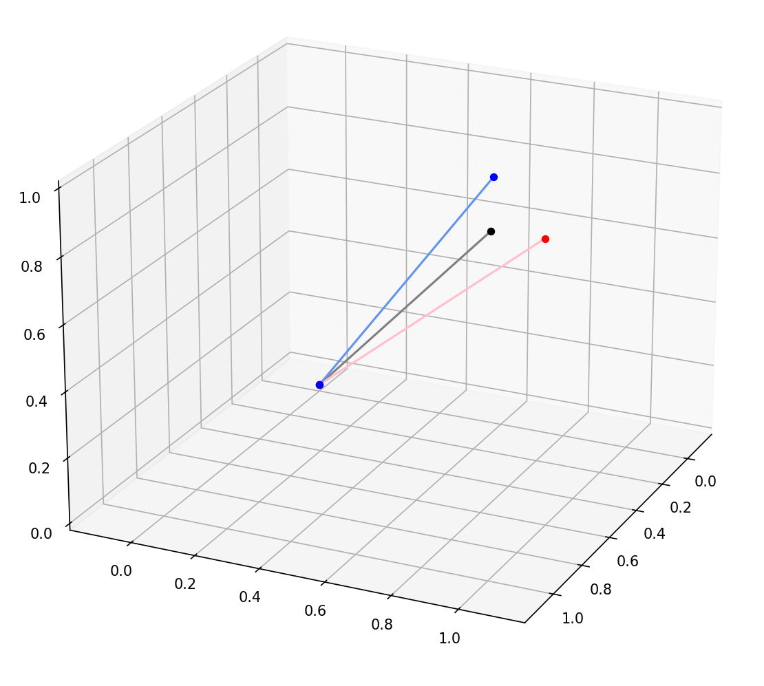
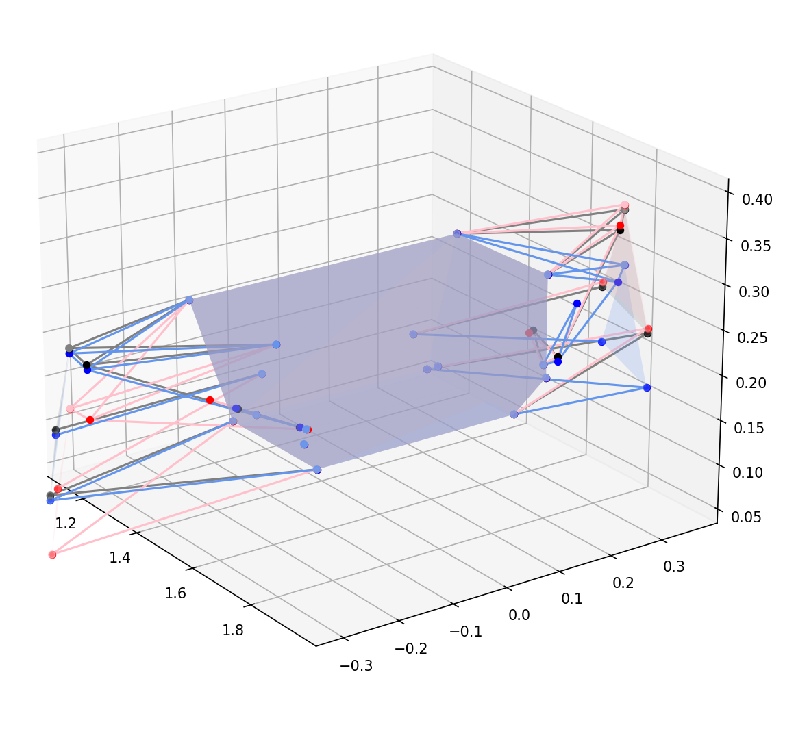
I tested this with the same simple system of a point fixed at the origin connected to a free point with a rigid link of known length, and my software was able to find both of these degrees of freedom in the system. It is also able to identify two degrees of freedom in a suspension with two wheels, one where each wheel moves down. To make the images below, I simply take the identified degrees of freedom and add them to the current \(\vec{q}\), and then plot the system with the new \(\vec{q}_{new} = \vec{q} + \delta \vec{q}\). The original system is in grey while the different degrees of freedom are in other colours.

How do we move in these degrees of freedom?

Here, we must continue to be aware of the intrinsic nonlinearities of the problem. Astute readers will notice that in the images above, the lengths of rigid links have changed. Simply stepping in the directions \(\delta q\) that we find in the previous part will not work, as each time our constraint functions will move slightly off zero. This could also change the shape of the constraint derivatives matrix, meaning that the next step that we take could also be in a wrong direction and could further make the values of the constraint functions deviate from zero. In physical terms, this means that our rigid links will end up stretching, which is highly undesirable. This idea is illustrated in the left side of the picture below. To solve this problem, we must do what is shown on the right side, and continously correct the constraint functions back to zero at each timestep.

To do this, note that we should not be stepping in the directions of our degrees of freedom. We should be altering \(\vec{q}\) in directions orthogonal to the degrees of freedom, as otherwise we will effectively create extra motion in the system, without making any progress towards correcting the values of the constraint function. Fortunately, we already have the vectors that make up the basis of this orthogonal space from SVD. Suppose that we identify k degrees of freedom from SVD. Then there are \((\text{num coords} - k)\) directions that we can move in that alter the constraint function. The k degrees of freedom will be the last \(k\) rows of \(V^*\), while these fixed directions will be the remaining rows of \(V^*\). Through the rest of this text, let these last k rows be the matrix \(D^*\) (D for degrees of freedom) and the remaining rows be \(F^*\) (F for fixed).

This correction step now reduces to the following problem:

\[\begin{gather*} \vec{f}(\vec{q} + \delta \vec{q}) = 0 \\ \delta \vec{q} = F \vec{x} \end{gather*}\]

Here, \(\vec{x}\) represents our perturbations in each of the valid deviations (the deviations orthogonal to the degrees of freedom). This problem is now a simple rootfinding problem, which we solve with Newton-Raphson. We can again use the Jacobian matrix \(J = \od{\vec{f}(\vec{q})}{\vec{q}}\) to write the Newton-Raphson update equation:

\[-J F \vec{x} = \vec{f}(\vec{q})\]

This is now a very simple Gaussian elimination problem, although in the underlying code I use np.linalg.lstsq to find the solution as this handles the edge case of a singular \(JF\) matrix.

How do we model forces and evaluate dynamics?

Common methods used for dynamics analysis in physics include Lagrangian and Hamiltonian methods (which I will definitely be experimenting with in the near future). However, I decided to use d'Alembert's principle as the central idea behind my dynamics simulation in this iteration. The central equation behind d'Alemberts is the following:

\[\sum_i (\dot{p_i} - F_i) \delta \vec{r}_i = 0\]

where \(\delta \vec{r}_i\) is a kinematically permissible virtual displacement in the coordinates. The idea is that from our previous work on evaluating degrees of freedom, we already know the values of \(\delta \vec{r}\)! The idea here is to generate a vector \(\vec{L}\) of the same dimensions as our state vector \(\vec{q}\) such that

\[\vec{L} \cdot \delta \vec{q} = \sum_i (\dot{p_i} - F_i) \delta \vec{r}_i = 0\]

This is quite easily doable. From our previous example where \(q_4, q_5, q_6\) are the X, Y and Z coordinates of the free point, if a force \(\vec{F}\) is applied to the free point, we can set \(L_4, L_5, L_6\) to be equal to \(-F_x, -F_y\) and \(-F_z\) respectively, and the equation above is satisfied.

If we know the forces on the car, this is quite easy to work with. However, there is some more work in finding \(\dot{p_i}\). To do this, I use a constant difference approximation to evaluate the change in the coordinates for constant acceleration in some timestep \(\Delta t\). This gives the following simple step update formula:

\[\vec{q}_{new} = \vec{q}(t + \Delta t) = \vec{q}(t) + \Delta t \dot{\vec{q}}(t) + \frac{\Delta t ^2}{2} \ddot{\vec{q}}(t)\]

By doing this, we can rearrange to evaluate \(\ddot{\vec{q}}\) as a function of \(\vec{q}_{new}\). Using the information on acceleration, we can calculate \(\dot{\vec{p}}_i = m\ddot{\vec{q}}_i\) for point masses. A much more involved calculation was required to implement more complicated masses like bars, but this is left as an exercise for the reader. As we also have \(\vec{F}_i\) as a function of \(\vec{q}_{new}\), we can write

\[\vec{L}(\vec{q}_{new}) \cdot \delta \vec{q} = 0\]

for all permissible variations \(\delta \vec{q}\). In fact, we can encapsulate all permissible variations from the degrees of freedom matrix \(D\) that we previously found to form the equation

\[\begin{gather*}\vec{L}(\vec{q}_{new})^{T} D = (0, 0, \dots 0) \\ D^T \vec{L}(\vec{q}_{new}) = \mathbf{0}\end{gather*}\]

This is just another rootfinding problem, which we can once again solve with Newton-Raphson. Note that for simplicity, I assume that \(\od{D}{\vec{q}} \approx 0\) for the calculation. The evaluation of \(\od{\vec{L}(\vec{q})}{\vec{q}}\) is still by no means elementary, and is difficult for bar masses and springs. Nonetheless, this work does not contribute to the overall idea behind the simulation and the work into this is once again left as an exercise to the reader ;). We can once again write \(\vec{q}_{new} = \vec{q} + \delta \vec{q}\) and then continue:

\[\begin{gather*}D^T \vec{L}(\vec{q} + \delta \vec{q}) = \mathbf{0} \\ D^T (\vec{L}(\vec{q}) + \od{\vec{L}(\vec{q})}{\vec{q}} D \vec{x}) = \mathbf{0} \\ D^T \od{\vec{L}(\vec{q})}{\vec{q}} D \vec{x} = -D^T \vec{L}(\vec{q}) \end{gather*}\]

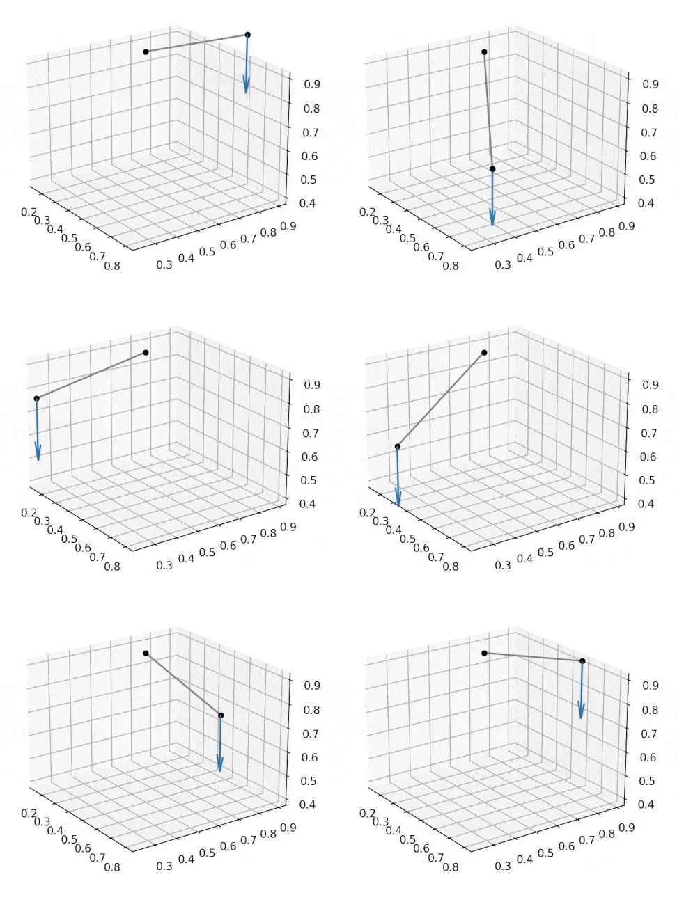
We can once again analytically calculate \(\od{\vec{L}(\vec{q})}{\vec{q}}\) (a lengthy but uninteresting process) and use numpy's least squares solution to solve for our new vector \(\vec{q}_{new}\). By doing this at every timestep (while making sure that we correct our q vectors as previously mentioned!), we can calculate the time evolution of the system. This is how the spring simulation below was created:

How do we evaluate constraint forces?

One key feature that I desired in this simulation was the ability to evaluate constraint forces. In this system, constraint forces are the forces on fixed points, or the forces of tension in rigid links. The mechanism of action of d'Alembert involves the fact that in a kinematically permissible variation, the work done by constraint forces is zero. For example, when we analyse the motion of a ball rolling along the floor, we never care about the normal reaction force from the floor since it will never ever perform any work. It turns out that the kinematically permissible variation statement is actually the secret to finding these forces.

When evaluating a constraint force, we can temporarily suppress the constraint equations that we are interested in evaluating. This will remove rows from \(\vec{f}(\vec{q})\), and will add new degrees of freedom. In the ball rolling on the floor example, this will add a degree of freedom where the ball can fall into the floor. Call this new degree of freedom matrix \(D_{aug}\). Our d'Alembert equation becomes \(L^T D_{aug} = \vec{e} \). However, \(\vec{e} \neq 0\). This is because there are now forces that were previously unaccounted for in the equation. We need to add forces to our \(L\) vector to take \(\vec{e}\) to zero! And these forces are our constraint forces! This can once again simply be solved with np.linalg.lstsq again.

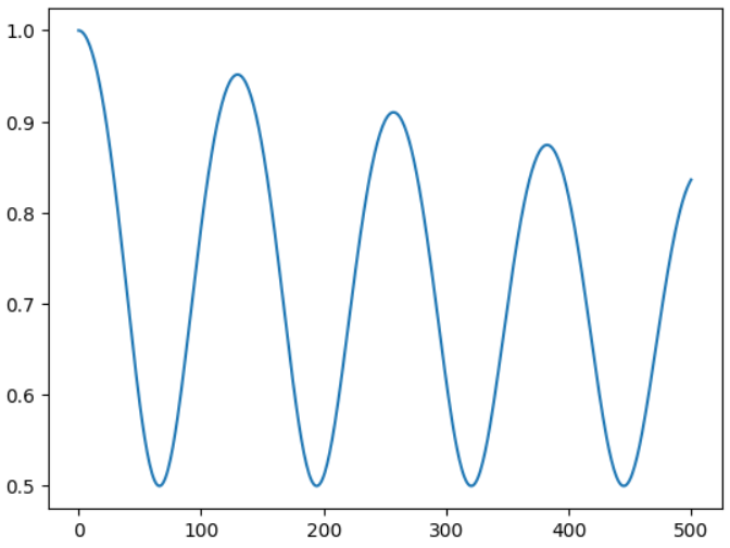
To demo this, I suspended a point mass from a rigid pendulum, and calculated the vertical force on the fixed point to plot the following graph:

Next steps and improvements

There is still a lot of work to be done in this simulation, and there are many ways to improve it.

SVD optimisation

The lowest hanging fruit here might be the SVD calculation, as the program appears to spend most time in this computation. As points are generally only constrained to a few others, the constraint equation matrix \(D\) is highly sparse. Methods do exist to exploit the sparsity of matrices in SVD, and using these could speed up the simulation process. There is also scope to reduce the number of coordinates used in the simulation heavily e.g. for rigid bodies, only the coordinates of three points can be used to reduce the size of the matrix (however, this idea will also significantly reduce the sparsity of the resulting matrix)

Work on the Newton Raphson steps

Many of the Newton-Raphson steps in this project occasionally fail to converge. For the Newton-Raphson used in the dynamics simulation, note the assumption made on the small value of \(\od{D}{\vec{q}}\). For the small pivots used in rocker geometry, D actually significantly varies with the motion of the coordinates. Calculating its derivative includes calculating the derivative of an SVD decomposition, which is possible yet is quite difficult and is also somewhat computationally expensive. It may be a good idea to look into non-analytic methods to locally evaluate the gradient and using a step size less aggresive than the effective one seen in Newton-Raphson to improve the rate of convergence, and also improve the ease in adding other features.

It is also probably a good idea to make the underlying method more equivalent to Euler backwards instead of Euler forwards i.e. switch to an implicit setup. Alternatively, a Runge-Kutta method with more steps could be used. This can help mitigate the energy losses that we see in this simulation (note the reducing forces seen in the plot above). A Hamiltonian setup could also help mitigate this.

Using a different strategy for dynamics

Using a Hamiltonian formulation for dynamics may actually be much easier than I previously thought. Watch this space!

---

Thank you for reading!